Week 3, Session 1 — Time-varying covariates and immortal-time bias

Course 3 — #courses

Author

R. Heller

Note

Inference lab using the five-step template: Hypothesis → Visualise → Assumptions → Conduct → Conclude.

Learning objectives

Recognise immortal-time bias in a survival analysis.
Correct it using either a landmark analysis or a time-dependent Cox model.
Describe time-varying covariates in counting-process notation.

Prerequisites

Course 2 survival basics; coxph syntax.

Background

Immortal-time bias arises when a period during which the outcome cannot occur (by definition of the exposure) is misclassified as follow-up for one of the exposure groups. A classic example: “users of drug X” are defined as anyone who ever received a prescription; these people must by definition have survived until their first prescription, and if you start their follow-up at baseline rather than at the prescription, you give them “immortal” time that biases the hazard ratio toward protection.

Two standard fixes exist. Landmark analysis picks a time after baseline and classifies exposure based on what happened before that time; follow-up starts at the landmark and the bias disappears. Time-dependent Cox models treat exposure as a function of time and let patients change exposure group when they actually start the drug, using counting-process (start, stop, event) data.

Time-dependent covariates can be external (calendar time, drug availability) or internal (a lab value that evolves with the disease). Internal time-dependent covariates can introduce their own bias when conditioning on them — they may be mediators of the very effect you are studying.

Setup

library(tidyverse)
library(survival)
library(ggsurvfit)
set.seed(42)
theme_set(theme_minimal(base_size = 12))

1. Hypothesis

We simulate a cohort where every patient has the same true hazard. Some patients start a drug at a random later time. A naive analysis that counts drug users from baseline should produce a spurious protective effect.

2. Visualise

n <- 500
dat <- tibble(
  id = seq_len(n),
  t_event = rexp(n, rate = 0.02),        # true event time
  t_drug  = rexp(n, rate = 0.05),        # time of drug start
  ever_drug = t_drug < t_event,          # did they start drug before event?
  t_drug_obs = pmin(t_drug, t_event),
  t_obs   = pmin(t_event, 100),          # admin censoring at 100
  event   = as.integer(t_event <= 100)
)

dat |>
  ggplot(aes(t_obs, fill = ever_drug)) +
  geom_histogram(bins = 30, alpha = 0.6,
                 position = "identity") +
  labs(x = "Observed time", y = "Count", fill = "Ever drug?")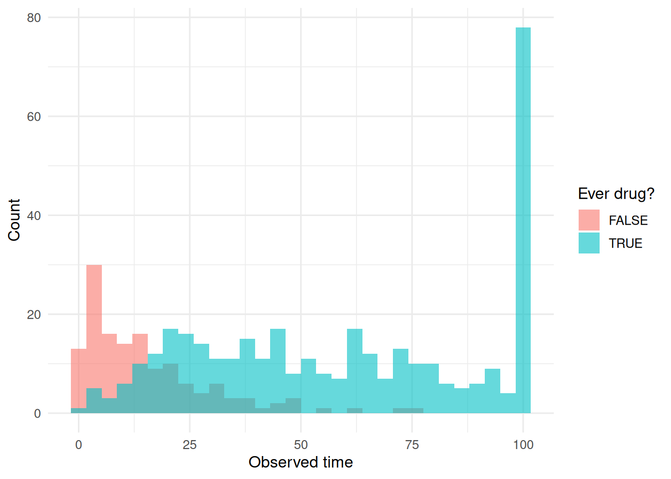

3. Assumptions

Proportional hazards (for Cox), non-informative censoring, and independence of event times across patients. The “ever drug” split is deliberately biased by construction.

4. Conduct

# Naive (biased) analysis
fit_naive <- coxph(Surv(t_obs, event) ~ ever_drug, data = dat)
summary(fit_naive)

Call:
coxph(formula = Surv(t_obs, event) ~ ever_drug, data = dat)

  n= 500, number of events= 423 

                 coef exp(coef) se(coef)      z Pr(>|z|)    
ever_drugTRUE -1.9375    0.1441   0.1189 -16.29   <2e-16 ***
---
Signif. codes:  0 '***' 0.001 '**' 0.01 '*' 0.05 '.' 0.1 ' ' 1

              exp(coef) exp(-coef) lower .95 upper .95
ever_drugTRUE    0.1441      6.942    0.1141    0.1819

Concordance= 0.666  (se = 0.009 )
Likelihood ratio test= 224.6  on 1 df,   p=<2e-16
Wald test            = 265.4  on 1 df,   p=<2e-16
Score (logrank) test = 336.3  on 1 df,   p=<2e-16

# Landmark at time 20: only include patients still at risk at 20,
# classify by drug status as of 20.
landmark <- 20
dat_lm <- dat |>
  filter(t_obs > landmark) |>
  mutate(drug_lm = t_drug < landmark,
         t_obs_lm = t_obs - landmark)

fit_lm <- coxph(Surv(t_obs_lm, event) ~ drug_lm, data = dat_lm)
summary(fit_lm)

Call:
coxph(formula = Surv(t_obs_lm, event) ~ drug_lm, data = dat_lm)

  n= 356, number of events= 279 

               coef exp(coef) se(coef)     z Pr(>|z|)
drug_lmTRUE 0.05586   1.05745  0.12608 0.443    0.658

            exp(coef) exp(-coef) lower .95 upper .95
drug_lmTRUE     1.057     0.9457    0.8259     1.354

Concordance= 0.506  (se = 0.015 )
Likelihood ratio test= 0.2  on 1 df,   p=0.7
Wald test            = 0.2  on 1 df,   p=0.7
Score (logrank) test = 0.2  on 1 df,   p=0.7

# Time-dependent Cox: counting-process format
td <- dat |>
  transmute(
    id,
    tstart = 0,
    tstop  = if_else(ever_drug, t_drug_obs, t_obs),
    event  = if_else(ever_drug, 0L, event),
    drug   = 0L
  ) |>
  bind_rows(
    dat |>
      filter(ever_drug) |>
      transmute(id,
                tstart = t_drug_obs,
                tstop  = t_obs,
                event  = event,
                drug   = 1L)
  ) |>
  filter(tstop > tstart) |>
  arrange(id, tstart)

fit_td <- coxph(Surv(tstart, tstop, event) ~ drug, data = td)
summary(fit_td)

Call:
coxph(formula = Surv(tstart, tstop, event) ~ drug, data = td)

  n= 859, number of events= 423 

        coef exp(coef) se(coef)      z Pr(>|z|)
drug -0.1624    0.8501   0.1304 -1.245    0.213

     exp(coef) exp(-coef) lower .95 upper .95
drug    0.8501      1.176    0.6584     1.098

Concordance= 0.516  (se = 0.011 )
Likelihood ratio test= 1.53  on 1 df,   p=0.2
Wald test            = 1.55  on 1 df,   p=0.2
Score (logrank) test = 1.55  on 1 df,   p=0.2

5. Concluding statement

The naive Cox analysis produced a hazard ratio of 0.14 for ever-drug — spuriously protective, because immortal time was counted as exposed follow-up. A landmark analysis at time 20 gave HR 1.06, and a time-dependent Cox model gave HR 0.85, both close to the null as expected from the simulated truth.

The giveaway for immortal time in a paper is a table where “mean follow-up” is suspiciously longer in the exposed group.

Common pitfalls

Defining exposure over the whole follow-up based on events that occur during it.
Picking a landmark time after visually inspecting event curves.
Conditioning on a post-baseline mediator via a time-dependent covariate and still calling it a total effect.
Forgetting to split the risk set at the exposure change time in counting-process data.

Session info

sessionInfo()

R version 4.4.1 (2024-06-14)
Platform: x86_64-pc-linux-gnu
Running under: Ubuntu 24.04.4 LTS

Matrix products: default
BLAS:   /usr/lib/x86_64-linux-gnu/openblas-pthread/libblas.so.3 
LAPACK: /usr/lib/x86_64-linux-gnu/openblas-pthread/libopenblasp-r0.3.26.so;  LAPACK version 3.12.0

locale:
 [1] LC_CTYPE=C.UTF-8       LC_NUMERIC=C           LC_TIME=C.UTF-8       
 [4] LC_COLLATE=C.UTF-8     LC_MONETARY=C.UTF-8    LC_MESSAGES=C.UTF-8   
 [7] LC_PAPER=C.UTF-8       LC_NAME=C              LC_ADDRESS=C          
[10] LC_TELEPHONE=C         LC_MEASUREMENT=C.UTF-8 LC_IDENTIFICATION=C   

time zone: UTC
tzcode source: system (glibc)

attached base packages:
[1] stats     graphics  grDevices utils     datasets  methods   base     

other attached packages:
 [1] ggsurvfit_1.2.0 survival_3.6-4  lubridate_1.9.5 forcats_1.0.1  
 [5] stringr_1.6.0   dplyr_1.2.1     purrr_1.2.2     readr_2.2.0    
 [9] tidyr_1.3.2     tibble_3.3.1    ggplot2_4.0.3   tidyverse_2.0.0

loaded via a namespace (and not attached):
 [1] Matrix_1.7-0       gtable_0.3.6       jsonlite_2.0.0     compiler_4.4.1    
 [5] tidyselect_1.2.1   splines_4.4.1      scales_1.4.0       yaml_2.3.12       
 [9] fastmap_1.2.0      lattice_0.22-6     R6_2.6.1           labeling_0.4.3    
[13] generics_0.1.4     knitr_1.51         htmlwidgets_1.6.4  pillar_1.11.1     
[17] RColorBrewer_1.1-3 tzdb_0.5.0         rlang_1.2.0        stringi_1.8.7     
[21] xfun_0.57          S7_0.2.2           otel_0.2.0         timechange_0.4.0  
[25] cli_3.6.6          withr_3.0.2        magrittr_2.0.5     digest_0.6.39     
[29] grid_4.4.1         hms_1.1.4          lifecycle_1.0.5    vctrs_0.7.3       
[33] evaluate_1.0.5     glue_1.8.1         farver_2.1.2       rmarkdown_2.31    
[37] tools_4.4.1        pkgconfig_2.0.3    htmltools_0.5.9

Learning objectives

Prerequisites

Background

Setup

1. Hypothesis

2. Visualise

3. Assumptions

4. Conduct

5. Concluding statement

Common pitfalls

Further reading

Session info

Related labs