Week 4, Session 3 — Survival primer: KM, log-rank, Cox PH

Course 2 — #courses

Author

R. Heller

Note

Inference lab: Hypothesis → Visualise → Assumptions → Conduct → Conclude.

Learning objectives

Estimate and plot a Kaplan-Meier survival curve for a two-group comparison.
Run and interpret a log-rank test.
Fit a Cox proportional-hazards model, check the PH assumption, and read a hazard ratio honestly.

Prerequisites

Comfort with GLMs and with reading a regression table.

Background

Survival analysis handles outcomes that are times to an event, where some subjects have not yet had the event when observation ends — the familiar right-censoring problem. Ignoring censoring by throwing out the censored observations biases the estimator; pretending the censored observations are event-free biases it the other way. The survival machinery handles censoring correctly by reasoning at each event time about who is still at risk.

Three tools cover most clinical applications: the Kaplan-Meier estimator for a non-parametric survival curve, the log-rank test for a two-group comparison, and Cox proportional-hazards regression for adjustment and multivariable modelling. The PH assumption — that the hazard ratio is constant over time — deserves explicit checking; when it fails, a time-varying coefficient or a stratified model is usually the right fix.

Setup

library(tidyverse)
library(survival)
library(ggsurvfit)
library(broom)
set.seed(42)
theme_set(theme_minimal(base_size = 12))

1. Hypothesis

Using survival::lung, compare survival between male and female patients. H₀: hazard ratio = 1. H₁: hazard ratio ≠ 1. α = 0.05.

2. Visualise

lung2 <- lung |>
  mutate(sex = factor(sex, levels = 1:2, labels = c("male", "female")))

km <- survfit2(Surv(time, status) ~ sex, data = lung2)

km |>
  ggsurvfit() +
  add_confidence_interval() +
  add_risktable() +
  labs(x = "Days", y = "Survival probability")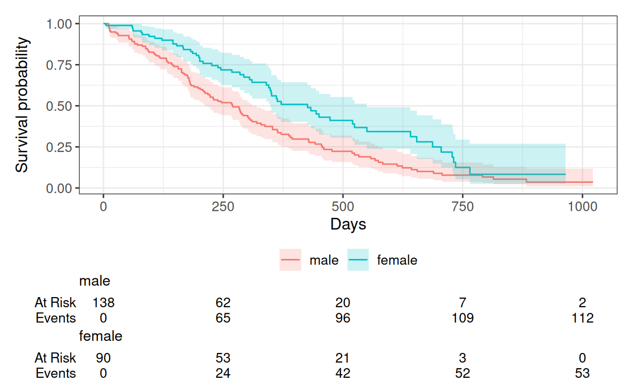

3. Assumptions

Two assumptions are worth checking: non-informative censoring (patients censored at a given time are representative of those still at risk) and proportional hazards.

cox_fit <- coxph(Surv(time, status) ~ sex + age, data = lung2)
cox.zph(cox_fit)

       chisq df    p
sex    2.608  1 0.11
age    0.209  1 0.65
GLOBAL 2.771  2 0.25

A large p-value on each row and a non-systematic Schoenfeld residual plot support the PH assumption; a small p calls for a time-varying coefficient or stratification.

4. Conduct

lr <- survdiff(Surv(time, status) ~ sex, data = lung2)
lr

Call:
survdiff(formula = Surv(time, status) ~ sex, data = lung2)

             N Observed Expected (O-E)^2/E (O-E)^2/V
sex=male   138      112     91.6      4.55      10.3
sex=female  90       53     73.4      5.68      10.3

 Chisq= 10.3  on 1 degrees of freedom, p= 0.001

tidy(cox_fit, exponentiate = TRUE, conf.int = TRUE)

# A tibble: 2 × 7
  term      estimate std.error statistic p.value conf.low conf.high
  <chr>        <dbl>     <dbl>     <dbl>   <dbl>    <dbl>     <dbl>
1 sexfemale    0.599   0.167       -3.06 0.00218    0.431     0.831
2 age          1.02    0.00922      1.85 0.0646     0.999     1.04

5. Concluding statement

Female sex was associated with a lower risk of death relative to male sex (HR 0.6; 95% CI 0.43 to 0.83; p = 0.0022), adjusted for age. The proportional-hazards assumption was not clearly violated (Schoenfeld test, all p > 0.05).

Emphasise the difference between a median survival comparison (which requires enough events) and a Cox model (which uses every event time).

Common pitfalls

Reporting a median survival that is not reached and calling it “undefined” in the results. Say so explicitly.
Ignoring the PH check because the output looks clean.
Comparing Kaplan-Meier curves by eye alone — add the log-rank test and the risk table.
Collapsing a competing event (e.g. death from another cause) into censoring without justification.

Session info

sessionInfo()

R version 4.4.1 (2024-06-14)
Platform: x86_64-pc-linux-gnu
Running under: Ubuntu 24.04.4 LTS

Matrix products: default
BLAS:   /usr/lib/x86_64-linux-gnu/openblas-pthread/libblas.so.3 
LAPACK: /usr/lib/x86_64-linux-gnu/openblas-pthread/libopenblasp-r0.3.26.so;  LAPACK version 3.12.0

locale:
 [1] LC_CTYPE=C.UTF-8       LC_NUMERIC=C           LC_TIME=C.UTF-8       
 [4] LC_COLLATE=C.UTF-8     LC_MONETARY=C.UTF-8    LC_MESSAGES=C.UTF-8   
 [7] LC_PAPER=C.UTF-8       LC_NAME=C              LC_ADDRESS=C          
[10] LC_TELEPHONE=C         LC_MEASUREMENT=C.UTF-8 LC_IDENTIFICATION=C   

time zone: UTC
tzcode source: system (glibc)

attached base packages:
[1] stats     graphics  grDevices utils     datasets  methods   base     

other attached packages:
 [1] broom_1.0.12    ggsurvfit_1.2.0 survival_3.6-4  lubridate_1.9.5
 [5] forcats_1.0.1   stringr_1.6.0   dplyr_1.2.1     purrr_1.2.2    
 [9] readr_2.2.0     tidyr_1.3.2     tibble_3.3.1    ggplot2_4.0.3  
[13] tidyverse_2.0.0

loaded via a namespace (and not attached):
 [1] Matrix_1.7-0       gtable_0.3.6       jsonlite_2.0.0     compiler_4.4.1    
 [5] tidyselect_1.2.1   splines_4.4.1      scales_1.4.0       yaml_2.3.12       
 [9] fastmap_1.2.0      lattice_0.22-6     R6_2.6.1           patchwork_1.3.2   
[13] labeling_0.4.3     generics_0.1.4     knitr_1.51         backports_1.5.1   
[17] htmlwidgets_1.6.4  pillar_1.11.1      RColorBrewer_1.1-3 tzdb_0.5.0        
[21] rlang_1.2.0        utf8_1.2.6         stringi_1.8.7      xfun_0.57         
[25] S7_0.2.2           otel_0.2.0         timechange_0.4.0   cli_3.6.6         
[29] withr_3.0.2        magrittr_2.0.5     digest_0.6.39      grid_4.4.1        
[33] hms_1.1.4          lifecycle_1.0.5    vctrs_0.7.3        evaluate_1.0.5    
[37] glue_1.8.1         farver_2.1.2       rmarkdown_2.31     tools_4.4.1       
[41] pkgconfig_2.0.3    htmltools_0.5.9

Learning objectives

Prerequisites

Background

Setup

1. Hypothesis

2. Visualise

3. Assumptions

4. Conduct

5. Concluding statement

Common pitfalls

Further reading

Session info

Related labs