library(tidyverse)
library(MASS)
set.seed(42)
theme_set(theme_minimal(base_size = 12))Week 1, Session 3 — PCA, factor analysis, CCA, LDA
Course 4 — #courses
Note
Workflow labs use the variant template: Goal → Approach → Execution → Check → Report.
Learning objectives
- Compute a PCA, read a biplot, and explain loadings and scores without resorting to magical reasoning about “directions of variance”.
- Distinguish PCA, factor analysis, canonical correlation analysis, and linear discriminant analysis by the question each answers.
- Fit an LDA classifier and interpret the discriminant coefficients.
Prerequisites
Matrix algebra from Course 1 (eigendecomposition); basic multivariate intuition.
Background
Dimension reduction is often described as “finding structure”, but each of these methods has a concrete question behind it. PCA asks which directions in feature space have the largest variance; its axes are eigenvectors of the covariance matrix. Factor analysis asks which latent factors, plus unique variance per feature, reproduce the observed covariance; it is PCA’s statistical cousin with a proper error model. Canonical correlation analysis asks which linear combinations of two feature sets are maximally correlated. Linear discriminant analysis asks which direction separates known classes while collapsing within-class variance.
They share machinery — all four involve eigenvalues of something — but they are not interchangeable. Using PCA where LDA was called for will waste the label information; using LDA where PCA was called for will produce a single, class-dependent axis and nothing else.
When you report a PCA, report the variance explained by each of the first few components and a biplot with named observations and loadings. When you report an LDA, report the classification accuracy on held-out data and the direction of each discriminant, not just the confusion matrix.
Setup
1. Goal
Use iris to illustrate PCA and LDA on the same data, compare their projections, and classify species with LDA.
2. Approach
Four morphometric variables, three species. PCA ignores the label; LDA uses it.
iris |>
  pivot_longer(-Species) |>
  ggplot(aes(value, fill = Species)) +
  geom_density(alpha = 0.5) +
  facet_wrap(~ name, scales = "free") +
  labs(x = NULL, y = "density")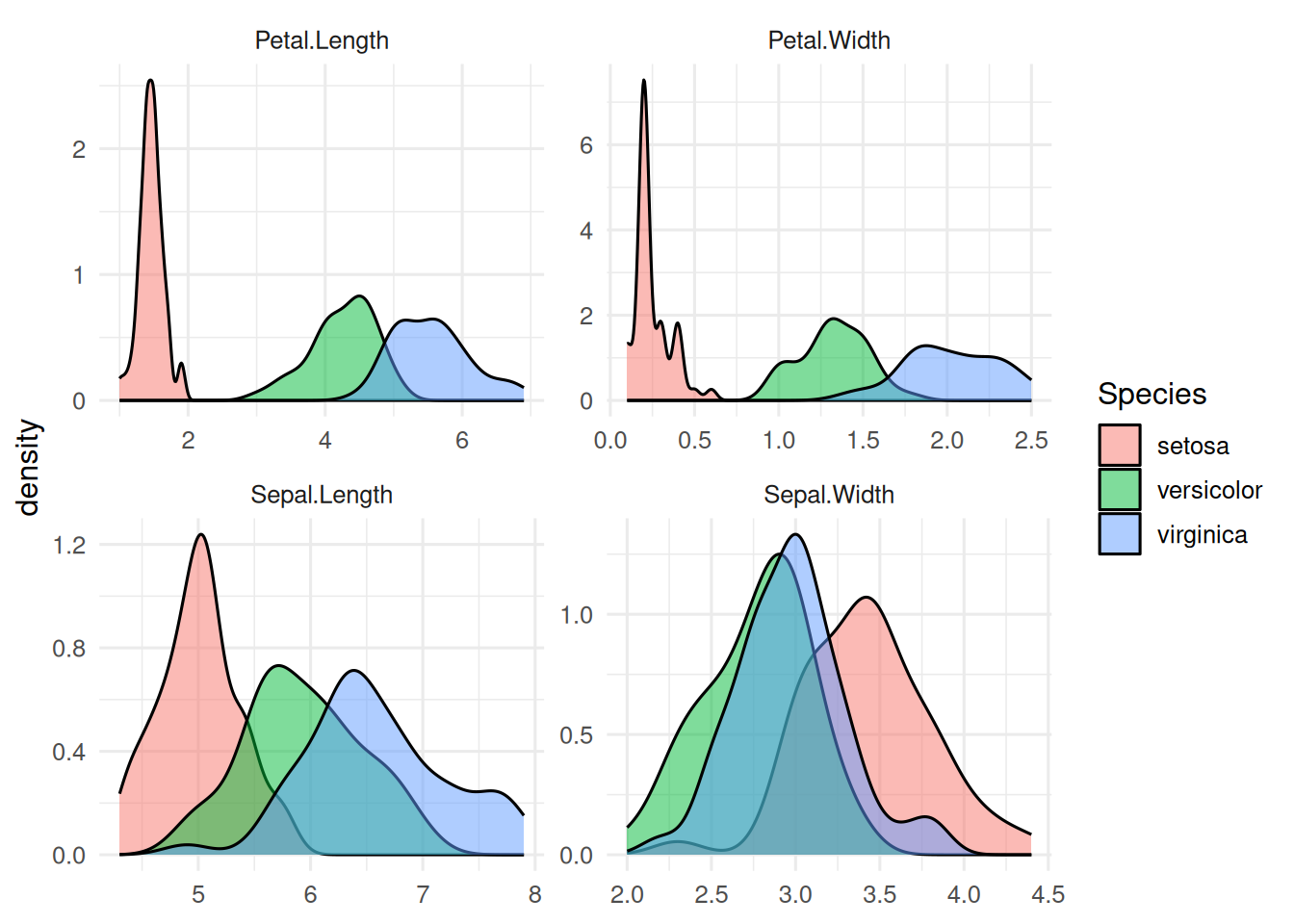
3. Execution
PCA on the four numeric features, then LDA.
pca <- prcomp(iris[, 1:4], scale. = TRUE)
summary(pca)$importance[, 1:3]
PC1 PC2 PC3
Standard deviation 1.708361 0.9560494 0.3830886
Proportion of Variance 0.729620 0.2285100 0.0366900
Cumulative Proportion 0.729620 0.9581300 0.9948200lda_fit <- lda(Species ~ ., data = iris)
lda_fit$scaling LD1 LD2
Sepal.Length 0.8293776 -0.02410215
Sepal.Width 1.5344731 -2.16452123
Petal.Length -2.2012117 0.93192121
Petal.Width -2.8104603 -2.83918785scores_pca <- as_tibble(pca$x[, 1:2]) |> mutate(Species = iris$Species)
scores_lda <- as_tibble(predict(lda_fit)$x) |> mutate(Species = iris$Species)
p1 <- ggplot(scores_pca, aes(PC1, PC2, colour = Species)) +
geom_point(alpha = 0.7) + labs(title = "PCA (unsupervised)")
p2 <- ggplot(scores_lda, aes(LD1, LD2, colour = Species)) +
geom_point(alpha = 0.7) + labs(title = "LDA (uses labels)")
gridExtra::grid.arrange(p1, p2, ncol = 2)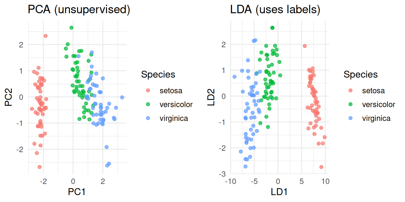
4. Check
Hold-out accuracy for LDA (simple 70/30 split).
idx <- sample(nrow(iris), 0.7 * nrow(iris))
fit2 <- lda(Species ~ ., data = iris[idx, ])
pred <- predict(fit2, iris[-idx, ])$class
mean(pred == iris$Species[-idx])
[1] 15. Report
On the iris data, the first two principal components explained 95.8% of the total variance. A linear discriminant classifier achieved hold-out accuracy of 100% on a 70/30 split.
In this low-dimensional problem, PCA already separates the species visually because the morphometric variables are correlated with species. In realistic biomedical data, that is rarely true: the supervised projection (LDA, or a classifier’s decision function) is usually sharper.
Skip factor analysis and CCA in the demo unless time permits; keep them as reading. The conceptual move — from unsupervised (PCA, FA) to supervised (LDA) to two-view (CCA) — is the point.
Common pitfalls
- Reporting “PC1 is age” because age happens to correlate with it.
- Running LDA when classes are hugely imbalanced; use QDA or a proper classifier instead.
- Comparing variance-explained across datasets as if it were a quality score.
Further reading
- Jolliffe IT (2002), Principal Component Analysis, 2nd ed.
- Mardia, Kent, Bibby, Multivariate Analysis, chapters on LDA/CCA.
Session info
sessionInfo()R version 4.5.2 (2025-10-31 ucrt)
Platform: x86_64-w64-mingw32/x64
Running under: Windows 11 x64 (build 26200)
Matrix products: default
LAPACK version 3.12.1
locale:
[1] LC_COLLATE=English_Germany.utf8 LC_CTYPE=English_Germany.utf8
[3] LC_MONETARY=English_Germany.utf8 LC_NUMERIC=C
[5] LC_TIME=English_Germany.utf8
time zone: Europe/Berlin
tzcode source: internal
attached base packages:
[1] stats graphics grDevices utils datasets methods base
other attached packages:
[1] MASS_7.3-65 lubridate_1.9.5 forcats_1.0.1 stringr_1.6.0
[5] dplyr_1.2.1 purrr_1.2.2 readr_2.2.0 tidyr_1.3.2
[9] tibble_3.3.1 ggplot2_4.0.3 tidyverse_2.0.0
loaded via a namespace (and not attached):
[1] gtable_0.3.6 jsonlite_2.0.0 compiler_4.5.2 tidyselect_1.2.1
[5] gridExtra_2.3 scales_1.4.0 yaml_2.3.12 fastmap_1.2.0
[9] R6_2.6.1 labeling_0.4.3 generics_0.1.4 knitr_1.51
[13] htmlwidgets_1.6.4 pillar_1.11.1 RColorBrewer_1.1-3 tzdb_0.5.0
[17] rlang_1.2.0 stringi_1.8.7 xfun_0.57 S7_0.2.2
[21] otel_0.2.0 timechange_0.4.0 cli_3.6.6 withr_3.0.2
[25] magrittr_2.0.4 digest_0.6.39 grid_4.5.2 hms_1.1.4
[29] lifecycle_1.0.5 vctrs_0.7.3 evaluate_1.0.5 glue_1.8.1
[33] farver_2.1.2 rmarkdown_2.31 tools_4.5.2 pkgconfig_2.0.3
[37] htmltools_0.5.9