library(tidyverse)
library(tidymodels)
library(MASS)
set.seed(42)
theme_set(theme_minimal(base_size = 12))Week 2, Session 5 — tidymodels pipelines
Course 4 — #courses
Note
Workflow labs use the variant template: Goal → Approach → Execution → Check → Report.
Learning objectives
- Build a
tidymodelsrecipe, workflow, and tuning grid for a binary classification task. - Split data for CV properly and collect metrics across resamples.
- Finalise a model on the full training data and evaluate on a test split.
Prerequisites
CV and regularisation from Week 1.
Background
tidymodels organises the modelling workflow into composable objects: a recipe describes preprocessing, a model specification describes the algorithm and its tunable parameters, a workflow bundles them, and tune functions drive resampling. The value of this separation is reproducibility: the same recipe runs on training, tuning, and test data, and it is hard to leak information across the split.
This lab builds a full pipeline on MASS::Pima.tr: logistic regression with elastic net and tuned mixture and penalty. The same pattern extends to random forests, boosting, neural networks, or any model with a parsnip wrapper.
The convention to remember: tune on the training folds, collect metrics, finalise with the best parameters, fit once to all of the training data, then evaluate once on the test set. The test set is touched exactly once.
Setup
1. Goal
Fit an elastic-net logistic regression to predict diabetes status on Pima.tr, using a proper tidymodels pipeline.
2. Approach
d <- as_tibble(MASS::Pima.tr)
ggplot(d, aes(glu, bmi, colour = type)) + geom_point(alpha = 0.7)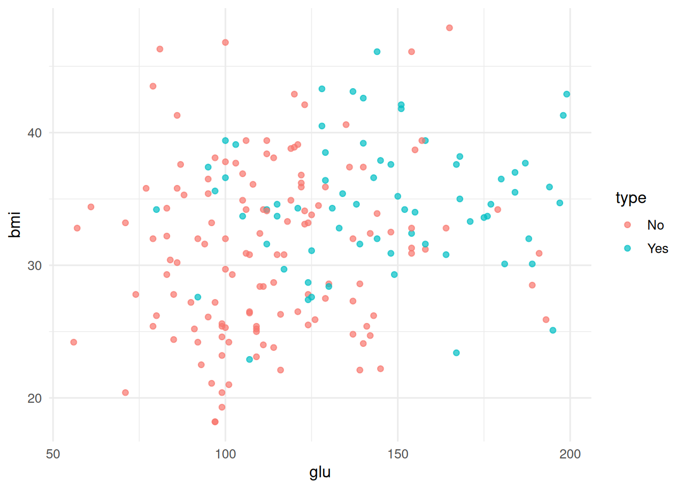
3. Execution
Split, recipe, model, workflow, tune.
d_split <- initial_split(d, prop = 0.75, strata = type)
d_train <- training(d_split); d_test <- testing(d_split)
folds <- vfold_cv(d_train, v = 5, strata = type)

rec <- recipe(type ~ ., data = d_train) |>
  step_normalize(all_numeric_predictors())

mod <- logistic_reg(penalty = tune(), mixture = tune()) |>
  set_engine("glmnet")

wf  <- workflow() |> add_recipe(rec) |> add_model(mod)

grid <- grid_regular(penalty(), mixture(), levels = 5)
res  <- tune_grid(wf, resamples = folds, grid = grid,
                  metrics = metric_set(roc_auc, accuracy))
collect_metrics(res) |>
  filter(.metric == "roc_auc") |>
  arrange(desc(mean)) |>
  head(5)
# A tibble: 5 × 8
penalty mixture .metric .estimator mean n std_err .config
<dbl> <dbl> <chr> <chr> <dbl> <int> <dbl> <chr>
1 0.00316 1 roc_auc binary 0.855 5 0.0305 pre0_mod20_post0
2 0.00316 0.25 roc_auc binary 0.853 5 0.0311 pre0_mod17_post0
3 0.00316 0.5 roc_auc binary 0.852 5 0.0304 pre0_mod18_post0
4 0.00316 0.75 roc_auc binary 0.852 5 0.0304 pre0_mod19_post0
5 0.0000000001 0 roc_auc binary 0.852 5 0.0328 pre0_mod01_post04. Check
Select best, finalise, evaluate on the test set.
best <- select_best(res, metric = "roc_auc")
wf_final <- finalize_workflow(wf, best)
fit_final <- fit(wf_final, data = d_train)
preds <- predict(fit_final, d_test, type = "prob") |>
  bind_cols(predict(fit_final, d_test), d_test)
roc_auc(preds, truth = type, .pred_Yes, event_level = "second")
# A tibble: 1 × 3
.metric .estimator .estimate
<chr> <chr> <dbl>
1 roc_auc binary 0.799accuracy(preds, truth = type, estimate = .pred_class)# A tibble: 1 × 3
.metric .estimator .estimate
<chr> <chr> <dbl>
1 accuracy binary 0.72roc_curve(preds, truth = type, .pred_Yes, event_level = "second") |>
autoplot()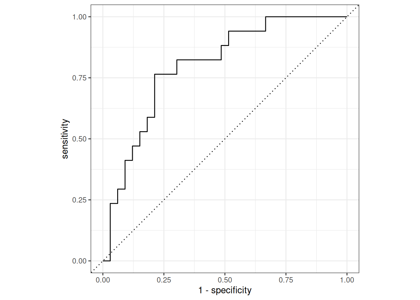
5. Report
An elastic-net logistic regression tuned on 5-fold CV, using a 5×5 grid over
penaltyandmixture, achieved a test ROC-AUC of 0.799 onMASS::Pima.tr.
The pipeline pattern — recipe + workflow + tune + finalise — is the template we will reuse for every predictive-model lab hereafter.
Show last_fit() as a one-liner for the finalise-then-evaluate step if time.
Common pitfalls
- Normalising the entire dataset before splitting; leakage is then baked in.
- Reporting the mean CV metric as if it were a test-set metric.
- Tuning without stratifying folds on an imbalanced outcome.
Further reading
- Kuhn M, Silge J, Tidy Modeling with R (online book).
Session info
sessionInfo()R version 4.5.2 (2025-10-31 ucrt)
Platform: x86_64-w64-mingw32/x64
Running under: Windows 11 x64 (build 26200)
Matrix products: default
LAPACK version 3.12.1
locale:
[1] LC_COLLATE=English_Germany.utf8 LC_CTYPE=English_Germany.utf8
[3] LC_MONETARY=English_Germany.utf8 LC_NUMERIC=C
[5] LC_TIME=English_Germany.utf8
time zone: Europe/Berlin
tzcode source: internal
attached base packages:
[1] stats graphics grDevices utils datasets methods base
other attached packages:
[1] MASS_7.3-65 yardstick_1.4.0 workflowsets_1.1.1 workflows_1.3.0
[5] tune_2.1.0 tailor_0.1.0 rsample_1.3.2 recipes_1.3.2
[9] parsnip_1.5.0 modeldata_1.5.1 infer_1.1.0 dials_1.4.3
[13] scales_1.4.0 broom_1.0.12 tidymodels_1.5.0 lubridate_1.9.5
[17] forcats_1.0.1 stringr_1.6.0 dplyr_1.2.1 purrr_1.2.2
[21] readr_2.2.0 tidyr_1.3.2 tibble_3.3.1 ggplot2_4.0.3
[25] tidyverse_2.0.0
loaded via a namespace (and not attached):
[1] tidyselect_1.2.1 timeDate_4052.112 farver_2.1.2
[4] S7_0.2.2 fastmap_1.2.0 digest_0.6.39
[7] rpart_4.1.27 timechange_0.4.0 lifecycle_1.0.5
[10] survival_3.8-6 magrittr_2.0.4 compiler_4.5.2
[13] rlang_1.2.0 tools_4.5.2 utf8_1.2.6
[16] yaml_2.3.12 data.table_1.18.2.1 knitr_1.51
[19] labeling_0.4.3 htmlwidgets_1.6.4 DiceDesign_1.10
[22] RColorBrewer_1.1-3 withr_3.0.2 nnet_7.3-20
[25] grid_4.5.2 sparsevctrs_0.3.6 future_1.70.0
[28] iterators_1.0.14 globals_0.19.1 cli_3.6.6
[31] rmarkdown_2.31 generics_0.1.4 otel_0.2.0
[34] rstudioapi_0.18.0 future.apply_1.20.2 tzdb_0.5.0
[37] splines_4.5.2 parallel_4.5.2 vctrs_0.7.3
[40] glmnet_5.0 hardhat_1.4.3 Matrix_1.7-5
[43] jsonlite_2.0.0 hms_1.1.4 listenv_0.10.1
[46] foreach_1.5.2 gower_1.0.2 glue_1.8.1
[49] parallelly_1.47.0 codetools_0.2-20 shape_1.4.6.1
[52] stringi_1.8.7 gtable_0.3.6 pillar_1.11.1
[55] furrr_0.4.0 htmltools_0.5.9 ipred_0.9-15
[58] lava_1.9.0 R6_2.6.1 evaluate_1.0.5
[61] lattice_0.22-9 backports_1.5.1 nanonext_1.9.0
[64] mirai_2.6.1 class_7.3-23 Rcpp_1.1.1-1.1
[67] prodlim_2026.03.11 xfun_0.57 pkgconfig_2.0.3