library(tidyverse)
library(glmnet)
set.seed(42)
theme_set(theme_minimal(base_size = 12))Week 1, Session 1 — Cross-validation, nested CV, bootstrap .632+
Course 4 — #courses
Note
Workflow labs use the variant template: Goal → Approach → Execution → Check → Report.
Learning objectives
- Implement k-fold and repeated k-fold cross-validation from scratch and with a package, and report an honest generalisation error.
- Explain why selecting a model and tuning a hyperparameter on the same fold inflates performance, and use nested CV to fix it.
- Compute a bootstrap .632+ estimate and say when it is preferable to
Prerequisites
Course 1 material on sampling variability; comfort with caret or base-R model fitting.
Background
Every predictive model reports an error on the data it was fit to. That number is almost always optimistic, because the fit has had a chance to memorise noise as well as signal. Cross-validation and the bootstrap are two resampling strategies that simulate the experience of scoring the model on data it has not seen. They are not interchangeable: they make different trade-offs between bias and variance, and they behave differently under high-dimensional settings.
A particular failure mode that recurs in the applied literature is double dipping: using the same held-out fold both to choose a hyperparameter and to report the final error. The fold is then no longer held out, and the reported error slides back toward the training error. Nested cross-validation is the clean solution: the inner loop picks hyperparameters, the outer loop reports error.
The bootstrap gives a different window onto generalisation. The plain bootstrap resamples with replacement; the .632 and .632+ variants combine apparent and out-of-bag errors. The .632+ correction adapts to estimated overfitting. Its bias and variance depend on the learner, loss, and data-generating process; no estimator is uniformly best.
A practical note: when you write up a modelling study, the generalisation error is the headline number. If you tuned, you must disclose how. If the inner tuning cost was hidden in the outer fold, a careful reader will notice that the reported error is too good and cannot be reproduced. Nested CV is not a cosmetic fix; it is the difference between a number that generalises and a number that does not.
Setup
1. Goal
Estimate the generalisation error of a lasso on a moderate p, small n simulated regression problem, first naively, then with a proper nested cross-validation.
2. Approach
We simulate n = 120 observations with p = 40 features, of which only 5 are true signal. We will (i) fit a single cv.glmnet, (ii) report the CV-minimising error, then (iii) wrap that in an outer 5-fold loop to show that the inner CV error is optimistic.
n <- 120; p <- 40
X <- matrix(rnorm(n * p), n, p)
beta <- c(rep(1.5, 5), rep(0, p - 5))
y <- as.numeric(X %*% beta + rnorm(n, sd = 1.0))

tibble(yhat_naive = as.numeric(X %*% beta), y = y) |>
  ggplot(aes(yhat_naive, y)) +
  geom_point(alpha = 0.6) +
  geom_abline(slope = 1, intercept = 0, colour = "grey50") +
  labs(x = "True linear predictor", y = "Observed y")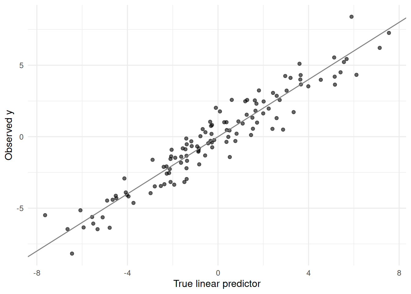
3. Execution
Naive single-layer CV.
cv1 <- cv.glmnet(X, y, alpha = 1, nfolds = 5)
naive_mse <- min(cv1$cvm)
naive_mse
[1] 1.206876Nested CV. The inner cv.glmnet picks lambda; the outer 5 folds produce the reported MSE.
K <- 5
folds <- sample(rep(1:K, length.out = n))
outer_mse <- numeric(K)
for (k in 1:K) {
  tr <- folds != k; te <- folds == k
  fit_k <- cv.glmnet(X[tr, ], y[tr], alpha = 1, nfolds = 5)
  yhat  <- as.numeric(predict(fit_k, newx = X[te, ], s = "lambda.min"))
  outer_mse[k] <- mean((y[te] - yhat)^2)
}
nested_mse <- mean(outer_mse)
c(naive = naive_mse, nested = nested_mse)
naive nested
1.206876 1.048175 4. Check
Bootstrap .632+ error as a cross-check.
# Apparent error uses the model trained on the original sample.
yhat_full <- as.numeric(predict(cv1, newx = X, s = "lambda.min"))
err_app <- mean((y - yhat_full)^2)
B <- 50
oob_loss <- matrix(NA_real_, nrow = n, ncol = B)
for (b in seq_len(B)) {
  idx <- sample.int(n, n, replace = TRUE)
  oob <- setdiff(seq_len(n), unique(idx))
  if (!length(oob)) next
  # Copies of the same observation stay together in the tuning folds.
  unique_idx <- unique(idx)
  boot_folds <- sample(rep(seq_len(5), length.out = length(unique_idx)))
  fit_b <- cv.glmnet(X[idx, ], y[idx], alpha = 1,
                     foldid = boot_folds[match(idx, unique_idx)])
  yhat_oob <- as.numeric(predict(fit_b, newx = X[oob, , drop = FALSE],
                                 s = "lambda.min"))
  oob_loss[oob, b] <- (y[oob] - yhat_oob)^2
}
stopifnot(all(rowSums(!is.na(oob_loss)) > 0))
# Average within observations first, so each observation has equal weight.
err_oob <- mean(rowMeans(oob_loss, na.rm = TRUE))
# No-information loss: all pairings of observed responses and fitted predictions.
gamma <- mean(outer(y, yhat_full, "-")^2)
bootstrap_errors <- function(apparent, oob, no_information) {
  stopifnot(all(is.finite(c(apparent, oob, no_information))),
            all(c(apparent, oob, no_information) >= 0))
  base <- 0.368 * apparent + 0.632 * oob
  bounded_oob <- min(oob, no_information)
  relative <- if (oob > apparent && no_information > apparent) {
    (bounded_oob - apparent) / (no_information - apparent)
  } else 0
  # Efron & Tibshirani (1997), equations 31-32: bounded correction.
  plus <- base + (bounded_oob - apparent) *
    0.368 * 0.632 * relative / (1 - 0.368 * relative)
  c(boot632 = base, boot632plus = plus, relative_overfit = relative)
}
boot_errors <- bootstrap_errors(err_app, err_oob, gamma)
err_632 <- unname(boot_errors["boot632"])
err_632plus <- unname(boot_errors["boot632plus"])
c(apparent = err_app, oob = err_oob, boot_errors, nested = nested_mse)
apparent oob boot632 boot632plus
0.73569350 1.22831749 1.04703186 1.05010707
relative_overfit nested
0.02657819 1.04817523 5. Report
On simulated data (n = 120, p = 40, five true signals), a lasso with tuning parameter chosen by 5-fold CV achieved an estimated MSE of 1.05 under nested 5 × 5 CV. The minimum single-layer CV estimate was 1.21; bootstrap .632 and .632+ estimates were 1.05 and 1.05, respectively.
The minimum inner-CV error is subject to selection optimism; its ordering relative to the outer estimate can vary in a single simulation. Outer CV keeps tuning separate from evaluation, but remains subject to sampling and fold variability. Here B = 50 keeps the demonstration small; assess Monte Carlo stability with more replicates before using bootstrap results in a study.
The .632+ calculation uses squared-error loss and the bounded correction in Efron and Tibshirani (1997), equations 26 and 31–32. Original observations are weighted equally in the out-of-bag estimate, and bootstrap duplicates are grouped in the inner tuning folds.
Emphasise that “naive CV” is still useful: it is the inner loop in a nested scheme. The crime is reporting it as the final error.
Common pitfalls
- Tuning on the test fold and reporting the resulting error.
- Using a single 80/20 split in high dimensions; variance across splits can exceed the effect of interest.
- Evaluating a bootstrap fit on its own training observations and calling that an out-of-sample error.
Further reading
- Hastie, Tibshirani, Friedman, Elements of Statistical Learning, §7.10–7.11.
- Varma S, Simon R (2006), Bias in error estimation when using cross-validation for model selection.
- Efron B, Tibshirani R (1997), Improvements on cross-validation: the .632+ bootstrap method.
Session info
sessionInfo()R version 4.6.1 (2026-06-24)
Platform: x86_64-pc-linux-gnu
Running under: Ubuntu 26.04.1 LTS
Matrix products: default
BLAS: /usr/lib/x86_64-linux-gnu/openblas-pthread/libblas.so.3
LAPACK: /usr/lib/x86_64-linux-gnu/openblas-pthread/libopenblasp-r0.3.32.so; LAPACK version 3.12.0
locale:
[1] LC_CTYPE=C.UTF-8 LC_NUMERIC=C LC_TIME=C.UTF-8
[4] LC_COLLATE=C.UTF-8 LC_MONETARY=C.UTF-8 LC_MESSAGES=C.UTF-8
[7] LC_PAPER=C.UTF-8 LC_NAME=C LC_ADDRESS=C
[10] LC_TELEPHONE=C LC_MEASUREMENT=C.UTF-8 LC_IDENTIFICATION=C
time zone: UTC
tzcode source: system (glibc)
attached base packages:
[1] stats graphics grDevices datasets utils methods base
other attached packages:
[1] glmnet_5.2 Matrix_1.7-5 lubridate_1.9.5 forcats_1.0.1
[5] stringr_1.6.0 dplyr_1.2.1 purrr_1.2.2 readr_2.2.0
[9] tidyr_1.3.2 tibble_3.3.1 ggplot2_4.0.3 tidyverse_2.0.0
loaded via a namespace (and not attached):
[1] generics_0.1.4 renv_1.3.1 shape_1.4.6.1 stringi_1.8.9
[5] lattice_0.22-9 hms_1.1.4 digest_0.6.39 magrittr_2.0.5
[9] evaluate_1.0.5 grid_4.6.1 timechange_0.4.0 RColorBrewer_1.1-3
[13] iterators_1.0.14 fastmap_1.2.0 foreach_1.5.2 jsonlite_2.0.0
[17] survival_3.8-6 scales_1.4.0 codetools_0.2-20 cli_3.6.6
[21] rlang_1.3.0 splines_4.6.1 withr_3.0.3 yaml_2.3.12
[25] otel_0.2.0 tools_4.6.1 tzdb_0.5.0 vctrs_0.7.3
[29] R6_2.6.1 lifecycle_1.0.5 htmlwidgets_1.6.4 pkgconfig_2.0.3
[33] pillar_1.11.1 gtable_0.3.6 glue_1.8.1 Rcpp_1.1.2
[37] xfun_0.62 tidyselect_1.2.1 knitr_1.52 farver_2.1.2
[41] htmltools_0.5.9 labeling_0.4.3 rmarkdown_2.32 compiler_4.6.1
[45] S7_0.2.2