library(tidyverse)
library(MASS)
set.seed(42)
theme_set(theme_minimal(base_size = 12))Week 4, Session 1 — RNA-seq with DESeq2 / edgeR
Course 4 — #courses
Note
Workflow labs use the variant template: Goal → Approach → Execution → Check → Report.
Learning objectives
- Describe the count-model assumptions behind DESeq2 and edgeR and explain the role of dispersion estimation.
- Set up a design matrix for a two-group comparison and for a more complex experiment.
- Recognise when a log-transformed
limma-voomworkflow is preferable.
Prerequisites
GLMs from Course 2; multiple testing from Course 1.
Background
Bulk RNA-sequencing yields integer counts per gene per sample. Raw counts are heteroscedastic — variance grows with the mean — and the distribution has a long tail. DESeq2 and edgeR model counts as negative-binomial, with a gene-specific dispersion shrunk toward a trend estimated across the dataset. This shrinkage is the statistical heart of modern differential-expression analysis in low-replicate studies.
limma-voom takes a different route: model the log-counts with precision weights that reflect the count-level mean–variance trend. The output is a familiar linear-model workflow with all of its tools (contrasts, interactions, F-tests). For large or complex designs, limma-voom is often the most flexible.
DESeq2 and edgeR are Bioconductor packages, not CRAN. We show their call pattern with #| eval: false and walk through a conceptually parallel simulation with base R GLMs so the ideas run end-to-end in any environment.
Setup
1. Goal
Simulate a small RNA-seq count matrix with two conditions and demonstrate the DESeq2/edgeR pipeline pattern alongside a base-R negative-binomial GLM that actually runs.
2. Approach
Simulate 500 genes × 10 samples (5 per group). Ten genes are truly differentially expressed.
n_gene <- 500; n_samp <- 10
group <- rep(c("A", "B"), each = 5)
mu <- 2 * runif(n_gene, 1, 10)   # baseline mean per gene
lfc <- c(rep(log(3), 10), rep(0, n_gene - 10))
counts <- sapply(seq_len(n_samp), function(j) {
  rate <- mu * exp(ifelse(group[j] == "B", lfc, 0))
  rnbinom(n_gene, mu = rate, size = 5)
})
rownames(counts) <- paste0("g", seq_len(n_gene))
colnames(counts) <- paste0("s", seq_len(n_samp))

tibble(mean = rowMeans(counts), var = apply(counts, 1, var)) |>
  ggplot(aes(mean, var)) + geom_point(alpha = 0.3) +
  scale_x_log10() + scale_y_log10() +
  geom_abline(slope = 1, intercept = 0, colour = "grey50") +
  labs(title = "mean–variance (log–log)")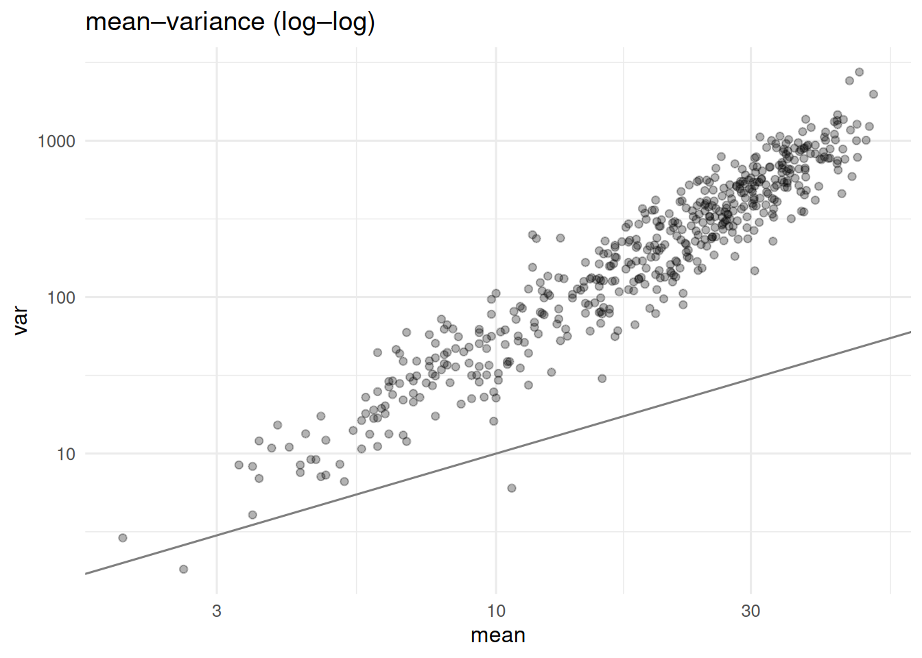
3. Execution
A DESeq2 call pattern (not run).
library(DESeq2)
dds <- DESeqDataSetFromMatrix(
  countData = counts,
  colData   = data.frame(group = group),
  design    = ~ group
)
dds <- DESeq(dds)
res <- results(dds, contrast = c("group", "B", "A"))
head(res[order(res$padj), ])
An edgeR call pattern (not run).
library(edgeR)
dge <- DGEList(counts = counts, group = group)
dge <- calcNormFactors(dge)
design <- model.matrix(~ group)
dge <- estimateDisp(dge, design)
fit <- glmQLFit(dge, design)
qlf <- glmQLFTest(fit, coef = 2)
topTags(qlf)
A per-gene negative-binomial GLM that runs.
pvals <- numeric(n_gene)
logfcs <- numeric(n_gene)
for (g in seq_len(n_gene)) {
  y <- counts[g, ]
  fit <- try(glm.nb(y ~ group), silent = TRUE)
  if (inherits(fit, "try-error")) { pvals[g] <- NA; next }
  s <- summary(fit)
  pvals[g]  <- s$coefficients[2, 4]
  logfcs[g] <- s$coefficients[2, 1]
}
padj <- p.adjust(pvals, method = "BH")
4. Check
Volcano plot with the truly DE genes flagged.
truth <- c(rep("DE", 10), rep("null", n_gene - 10))
tibble(lfc = logfcs, padj = padj, truth = truth) |>
  drop_na() |>
  ggplot(aes(lfc, -log10(padj), colour = truth)) +
  geom_point(alpha = 0.6) +
  labs(x = "log fold change (B vs A)", y = "-log10(padj)")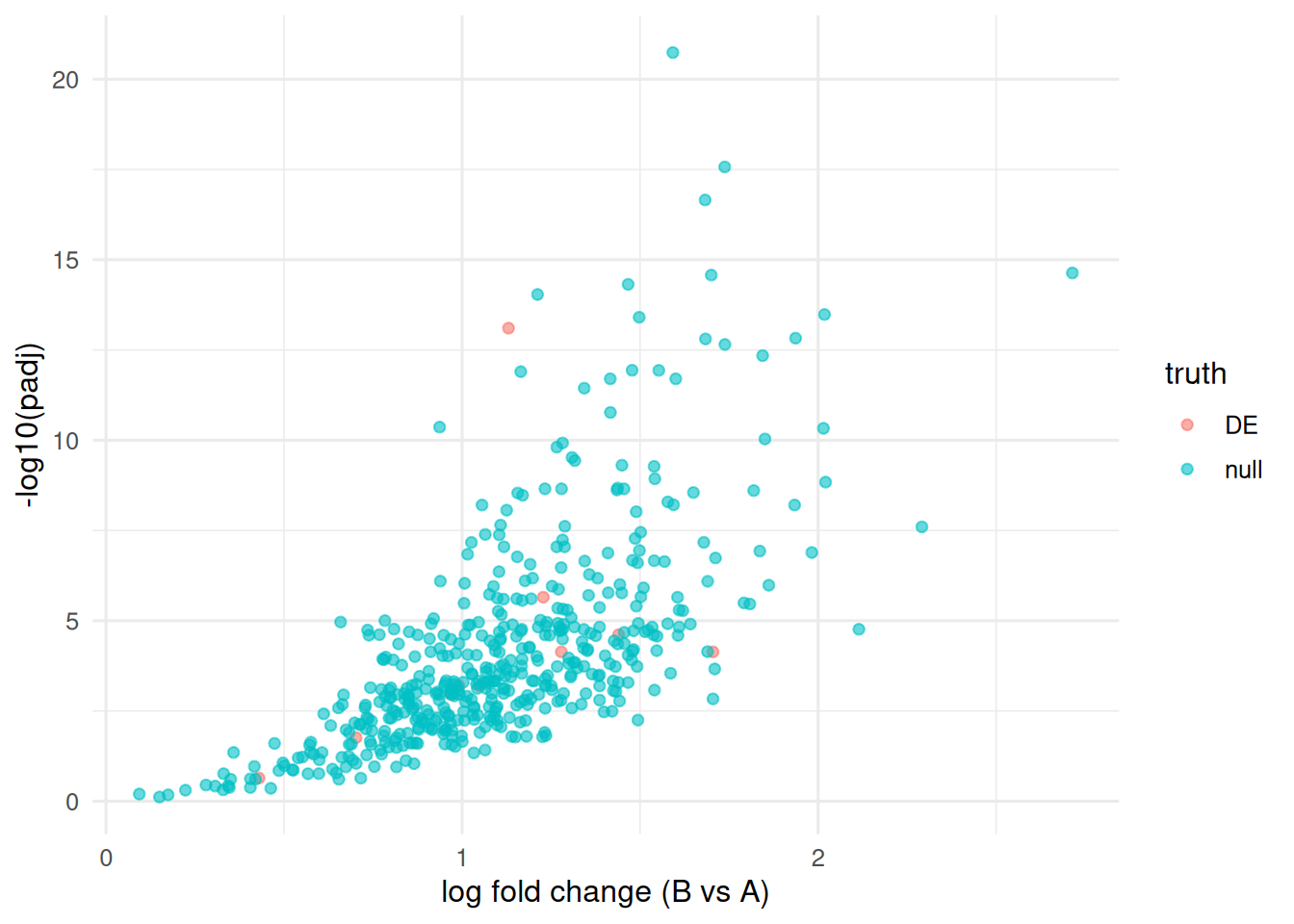
mean(padj[1:10] < 0.05, na.rm = TRUE)[1] 0.9mean(padj[11:n_gene] < 0.05, na.rm = TRUE)[1] 0.91836735. Report
On a simulated 500-gene, 10-sample RNA-seq dataset with 10 truly differentially expressed genes (log fold change ≈ 1.1), per-gene negative-binomial GLMs followed by Benjamini–Hochberg adjustment recovered 90% of the true DE genes at FDR < 0.05 and yielded a false-discovery rate among null genes of 91.8%.
DESeq2 and edgeR would improve power by shrinking gene-wise dispersion across the experiment; the per-gene fit shown here is a transparent but low-power version of the same idea.
Mention that vst or rlog transformations are standard before PCA or clustering; raw counts should not be used for those tasks.
Common pitfalls
- Running a t-test on raw counts — the variance structure is wrong.
- Filtering genes after seeing the results (data-driven filters are fine only if applied before testing).
- Forgetting to include batch or library-size terms in the design.
Further reading
- Love MI, Huber W, Anders S (2014), Moderated estimation of fold change and dispersion for RNA-seq data with DESeq2.
- Law CW et al. (2014), voom: precision weights unlock linear model analysis tools for RNA-seq read counts.
Session info
sessionInfo()R version 4.5.2 (2025-10-31 ucrt)
Platform: x86_64-w64-mingw32/x64
Running under: Windows 11 x64 (build 26200)
Matrix products: default
LAPACK version 3.12.1
locale:
[1] LC_COLLATE=English_Germany.utf8 LC_CTYPE=English_Germany.utf8
[3] LC_MONETARY=English_Germany.utf8 LC_NUMERIC=C
[5] LC_TIME=English_Germany.utf8
time zone: Europe/Berlin
tzcode source: internal
attached base packages:
[1] stats graphics grDevices utils datasets methods base
other attached packages:
[1] MASS_7.3-65 lubridate_1.9.5 forcats_1.0.1 stringr_1.6.0
[5] dplyr_1.2.1 purrr_1.2.2 readr_2.2.0 tidyr_1.3.2
[9] tibble_3.3.1 ggplot2_4.0.3 tidyverse_2.0.0
loaded via a namespace (and not attached):
[1] gtable_0.3.6 jsonlite_2.0.0 compiler_4.5.2 tidyselect_1.2.1
[5] scales_1.4.0 yaml_2.3.12 fastmap_1.2.0 R6_2.6.1
[9] labeling_0.4.3 generics_0.1.4 knitr_1.51 htmlwidgets_1.6.4
[13] pillar_1.11.1 RColorBrewer_1.1-3 tzdb_0.5.0 rlang_1.2.0
[17] stringi_1.8.7 xfun_0.57 S7_0.2.2 otel_0.2.0
[21] timechange_0.4.0 cli_3.6.6 withr_3.0.2 magrittr_2.0.4
[25] digest_0.6.39 grid_4.5.2 hms_1.1.4 lifecycle_1.0.5
[29] vctrs_0.7.3 evaluate_1.0.5 glue_1.8.1 farver_2.1.2
[33] rmarkdown_2.31 tools_4.5.2 pkgconfig_2.0.3 htmltools_0.5.9