---
title: "Nash's existence theorem: fixed-point proof and computation"
description: "Trace Nash's 1950 existence proof for equilibria in finite games using Kakutani's fixed-point theorem, implement the best-response correspondence in R, visualise the fixed-point mapping for 2×2 games, and connect the proof structure to modern equilibrium computation."
author: "Raban Heller"
date: 2026-05-08
date-modified: 2026-05-08
categories:
- history-of-gt-mathematics
- nash-equilibrium
- fixed-point-theorems
- existence-proofs
keywords: ["Nash existence theorem", "Kakutani fixed point", "Brouwer fixed point", "best-response correspondence", "equilibrium existence"]
labels: ["history-of-gt", "equilibrium-theory"]
tier: 1
bibliography: ../../../references.bib
vgwort: "TODO_VGWORT_history-of-gt-mathematics_nash-existence-proof"
image: thumbnail.png
image-alt: "Best-response correspondence mapping in a 2×2 game showing the fixed point where both players' best responses intersect at Nash equilibrium"
citation:
type: webpage
url: https://cttir.github.io/equilibria/tutorials/history-of-gt-mathematics/nash-existence-proof/
license: "CC BY-SA 4.0"
draft: false
has_static_fig: true
has_interactive_fig: true
has_shiny_app: false
---
```{r}
#| label: setup
#| include: false
library(ggplot2)
library(dplyr)
library(tidyr)
library(plotly)
okabe_ito <- c("#E69F00", "#56B4E9", "#009E73", "#F0E442",
"#0072B2", "#D55E00", "#CC79A7", "#999999")
theme_publication <- function(base_size = 12) {
theme_minimal(base_size = base_size) +
theme(plot.title = element_text(size = base_size * 1.2, face = "bold"),
plot.subtitle = element_text(size = base_size * 0.9, color = "grey40"),
axis.line = element_line(color = "grey30", linewidth = 0.3),
panel.grid.minor = element_blank(), legend.position = "bottom",
plot.margin = margin(10, 10, 10, 10))
}
```
## Introduction & motivation
John Nash's 1950 proof that every finite game possesses at least one equilibrium in mixed strategies is one of the most consequential results in the social sciences. The theorem guarantees that for any game with finitely many players, each choosing from finitely many pure strategies, there exists a strategy profile where no player can improve their expected payoff by unilaterally deviating. This existence guarantee transforms game theory from a collection of special cases into a general theory: no matter how complex the strategic interaction, an equilibrium exists.
Nash's proof is remarkably concise — his 1950 Proceedings of the National Academy of Sciences paper is barely one page — and relies on Kakutani's fixed-point theorem applied to the best-response correspondence. The key insight is that finding an equilibrium is equivalent to finding a fixed point of a particular mapping from the space of strategy profiles to itself. Each player's best-response correspondence maps the other players' strategies to the set of optimal replies. The product of these correspondences maps the full strategy space to itself, and Kakutani's theorem guarantees that this mapping has a fixed point — a profile where every player is simultaneously best-responding to the others.
The proof's elegance masks deep computational implications. While Nash proved that equilibria exist, his proof is non-constructive: it tells us a fixed point is there but not how to find it. This gap between existence and computation has driven fifty years of algorithmic game theory. The Lemke-Howson algorithm (1964) provides a constructive path to Nash equilibrium in two-player games, but its worst-case running time is exponential. The PPAD-completeness results of Daskalakis, Goldberg, and Papadimitriou (2009) show that this is likely inherent: finding a Nash equilibrium is computationally hard in general, even though we know one exists. This tutorial reconstructs Nash's argument computationally, implementing the best-response correspondence and visualising why the fixed point must exist.
Understanding the proof also illuminates what Nash equilibrium is and is not. The fixed-point argument applies to mixed strategies over a compact, convex strategy space. Pure-strategy equilibria may or may not exist — the guarantee is only for mixed extensions. The proof requires finite strategy sets (or compact strategy spaces with continuous payoffs in the infinite case). And the fixed-point structure reveals that Nash equilibrium is fundamentally a consistency condition: a profile is an equilibrium precisely when the best-response mapping sends it to itself.
## Mathematical formulation
**Setting**: A finite game $\Gamma = (N, (S_i)_{i \in N}, (u_i)_{i \in N})$ with $n$ players, each with finite strategy set $S_i$ and payoff function $u_i: \prod_j S_j \to \mathbb{R}$.
**Mixed extension**: Player $i$'s mixed strategy is $\sigma_i \in \Delta(S_i)$, the probability simplex over $S_i$. The mixed strategy space is $\Sigma = \prod_i \Delta(S_i)$.
**Best-response correspondence**: For player $i$, given $\sigma_{-i}$:
$$BR_i(\sigma_{-i}) = \arg\max_{\sigma_i \in \Delta(S_i)} u_i(\sigma_i, \sigma_{-i})$$
**Product correspondence**: $BR(\sigma) = \prod_i BR_i(\sigma_{-i})$ maps $\Sigma \to 2^{\Sigma}$.
**Kakutani's theorem**: If $\Sigma$ is compact and convex, and $BR: \Sigma \to 2^{\Sigma}$ has nonempty, convex values and a closed graph, then $\exists\, \sigma^* \in \Sigma$ with $\sigma^* \in BR(\sigma^*)$.
**Verification**: (1) $\Sigma$ is a product of simplices — compact and convex. (2) $BR_i(\sigma_{-i})$ is the set of maximisers of a linear function over a simplex — nonempty and convex. (3) The graph $\{(\sigma, \tau) : \tau \in BR(\sigma)\}$ is closed because payoffs are continuous in mixed strategies. Therefore, a fixed point $\sigma^*$ exists, which is a Nash equilibrium.
## R implementation
```{r}
#| label: nash-existence
set.seed(42)

cat("=== Nash Existence: Fixed-Point Computation ===\n\n")
# === Best-response correspondence for 2×2 games ===
best_response_row <- function(A, q) {
  # A = row player payoff matrix, q = P(Left) for column player
  eu_top <- A[1,1]*q + A[1,2]*(1-q)
  eu_bot <- A[2,1]*q + A[2,2]*(1-q)
  if (eu_top > eu_bot + 1e-10) return(1.0)
  if (eu_bot > eu_top + 1e-10) return(0.0)
  return(0.5)  # indifferent — return midpoint of BR set
}

best_response_col <- function(B, p) {
  eu_left <- B[1,1]*p + B[2,1]*(1-p)
  eu_right <- B[1,2]*p + B[2,2]*(1-p)
  if (eu_left > eu_right + 1e-10) return(1.0)
  if (eu_right > eu_left + 1e-10) return(0.0)
  return(0.5)
}

# === Fixed-point iteration (smoothed best response) ===
smoothed_br <- function(payoffs, opp_prob, lambda = 20) {
  eu <- payoffs * c(opp_prob, 1 - opp_prob)
  eu_strat <- c(sum(payoffs[1,] * c(opp_prob, 1-opp_prob)),
                sum(payoffs[2,] * c(opp_prob, 1-opp_prob)))
  exp_eu <- exp(lambda * eu_strat)
  exp_eu[1] / sum(exp_eu)
}

# === Game: Battle of the Sexes ===
A_bos <- matrix(c(3, 0, 0, 2), 2, 2)
B_bos <- matrix(c(2, 0, 0, 3), 2, 2)

cat("--- Battle of the Sexes ---\n")
cat("Row payoffs:\n")
print(A_bos)
cat("Col payoffs:\n")
print(B_bos)
# Trace fixed-point iteration
p <- 0.5; q <- 0.5
trajectory <- data.frame(iter = 0, p = p, q = q)
for (i in 1:50) {
  p_new <- smoothed_br(A_bos, q, lambda = 5)
  q_new <- smoothed_br(t(B_bos), p, lambda = 5)
  p <- p_new; q <- q_new
  trajectory <- rbind(trajectory, data.frame(iter = i, p = p, q = q))
}
cat(sprintf("\nSmoothed BR iteration (λ=5): converges to p=%.4f, q=%.4f\n", p, q))
# === Analytical NE for 2×2 games ===
find_mixed_ne <- function(A, B) {
  # Mixed NE: column indifferent => q* solves A[1,1]q + A[1,2](1-q) = A[2,1]q + A[2,2](1-q)
  denom_p <- (A[1,1] - A[1,2] - A[2,1] + A[2,2])
  denom_q <- (B[1,1] - B[1,2] - B[2,1] + B[2,2])
  q_star <- if (abs(denom_p) > 1e-10) (A[2,2] - A[1,2]) / denom_p else NA
  p_star <- if (abs(denom_q) > 1e-10) (B[2,2] - B[1,2]) / denom_q else NA
  c(p = p_star, q = q_star)
}

ne <- find_mixed_ne(A_bos, B_bos)
cat(sprintf("Analytical mixed NE: p=%.4f, q=%.4f\n", ne["p"], ne["q"]))
# === Test on multiple random games ===
cat("\n--- Fixed-Point Convergence on Random Games ---\n")
n_games <- 100
converged <- 0
for (g in 1:n_games) {
  A <- matrix(runif(4, -5, 5), 2, 2)
  B <- matrix(runif(4, -5, 5), 2, 2)
  p <- runif(1); q <- runif(1)
  for (i in 1:200) {
    p <- smoothed_br(A, q, lambda = 10)
    q <- smoothed_br(t(B), p, lambda = 10)
  }
  # Check approximate equilibrium
  eu_top <- A[1,1]*q + A[1,2]*(1-q)
  eu_bot <- A[2,1]*q + A[2,2]*(1-q)
  eu_left <- B[1,1]*p + B[2,1]*(1-p)
  eu_right <- B[1,2]*p + B[2,2]*(1-p)
  regret_r <- max(eu_top, eu_bot) - (p*eu_top + (1-p)*eu_bot)
  regret_c <- max(eu_left, eu_right) - (q*eu_left + (1-q)*eu_right)
  if (max(regret_r, regret_c) < 0.1) converged <- converged + 1
}
cat(sprintf("  %d/%d random 2×2 games: smoothed BR found ε<0.1 equilibrium\n",
            converged, n_games))
```
## Static publication-ready figure
```{r}
#| label: fig-best-response
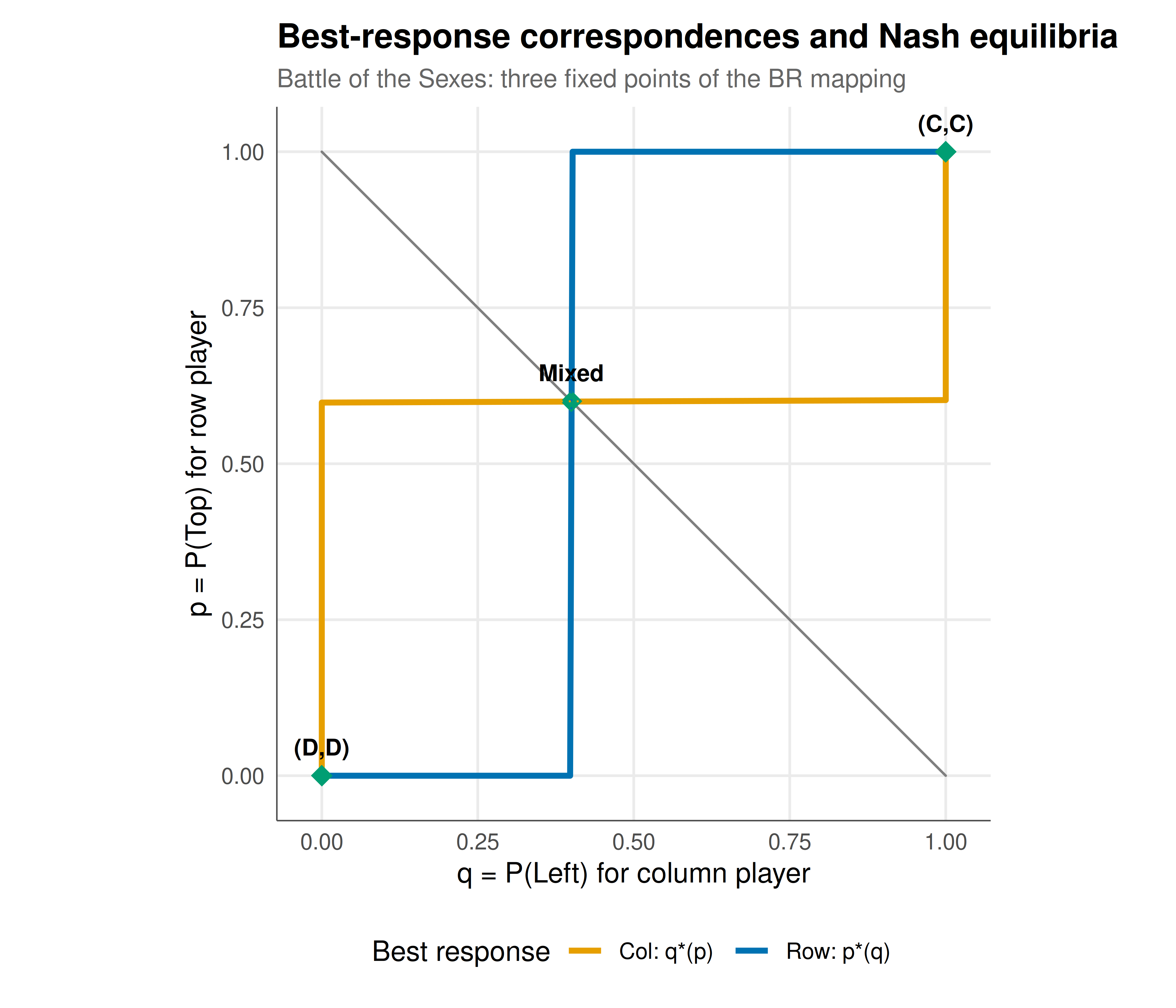
#| fig-cap: "Figure 1. Best-response correspondences for the Battle of the Sexes game. The blue step function shows row player's best response p*(q) as a function of column's mixing probability q. The orange step function shows column player's best response q*(p) as a function of row's mixing probability p. Nash equilibria occur at intersections of the two correspondences: two pure-strategy equilibria at the corners (0,0) and (1,1), and one mixed equilibrium near (0.6, 0.4). The smoothed best-response trajectory (dashed grey) spirals toward the mixed equilibrium from the centre. Okabe-Ito palette."
#| dev: [png, pdf]
#| fig-width: 7
#| fig-height: 6
#| dpi: 300
# Best-response correspondences for BoS
q_grid <- seq(0, 1, length.out = 501)
p_grid <- seq(0, 1, length.out = 501)

br_row <- sapply(q_grid, function(q) best_response_row(A_bos, q))
br_col <- sapply(p_grid, function(p) best_response_col(B_bos, p))

br_data <- bind_rows(
  tibble(x = q_grid, y = br_row, player = "Row: p*(q)"),
  tibble(x = br_col, y = p_grid, player = "Col: q*(p)")
)

# Indifference points
q_indiff <- (A_bos[2,2] - A_bos[1,2]) / (A_bos[1,1] - A_bos[1,2] - A_bos[2,1] + A_bos[2,2])
p_indiff <- (B_bos[2,2] - B_bos[1,2]) / (B_bos[1,1] - B_bos[1,2] - B_bos[2,1] + B_bos[2,2])

ne_points <- tibble(
  q = c(0, 1, q_indiff),
  p = c(0, 1, p_indiff),
  label = c("(D,D)", "(C,C)", "Mixed")
)

ggplot() +
  geom_path(data = br_data |> filter(player == "Row: p*(q)"),
            aes(x = x, y = y, color = player), linewidth = 1.2) +
  geom_path(data = br_data |> filter(player == "Col: q*(p)"),
            aes(x = x, y = y, color = player), linewidth = 1.2) +
  geom_path(data = trajectory, aes(x = q, y = p),
            color = "grey50", linetype = "dashed", linewidth = 0.5) +
  geom_point(data = ne_points, aes(x = q, y = p), size = 4, shape = 18,
             color = okabe_ito[3]) +
  geom_text(data = ne_points, aes(x = q, y = p, label = label),
            vjust = -1.2, size = 3.5, fontface = "bold") +
  geom_segment(aes(x = q_indiff, xend = q_indiff, y = 0, yend = 1),
               linetype = "dotted", color = okabe_ito[5], linewidth = 0.4) +
  geom_segment(aes(x = 0, xend = 1, y = p_indiff, yend = p_indiff),
               linetype = "dotted", color = okabe_ito[1], linewidth = 0.4) +
  scale_color_manual(values = c("Row: p*(q)" = okabe_ito[5],
                                 "Col: q*(p)" = okabe_ito[1]),
                     name = "Best response") +
  labs(title = "Best-response correspondences and Nash equilibria",
       subtitle = "Battle of the Sexes: three fixed points of the BR mapping",
       x = "q = P(Left) for column player",
       y = "p = P(Top) for row player") +
  coord_equal(xlim = c(-0.02, 1.02), ylim = c(-0.02, 1.02)) +
  theme_publication()
```
## Interactive figure
```{r}
#| label: fig-convergence-interactive
# Convergence of smoothed BR across different lambda values
lambdas <- c(2, 5, 10, 20)
conv_data <- lapply(lambdas, function(lam) {
  p <- 0.5; q <- 0.5
  traj <- tibble(iter = 0, p = p, q = q, lambda = lam,
                 dist = sqrt((p - p_indiff)^2 + (q - q_indiff)^2))
  for (i in 1:80) {
    p <- smoothed_br(A_bos, q, lambda = lam)
    q <- smoothed_br(t(B_bos), p, lambda = lam)
    d <- sqrt((p - p_indiff)^2 + (q - q_indiff)^2)
    traj <- bind_rows(traj, tibble(iter = i, p = p, q = q, lambda = lam, dist = d))
  }
  traj
}) |> bind_rows() |>
  mutate(lambda_label = paste0("λ = ", lambda),
         text = paste0("Iteration: ", iter,
                       "\nλ = ", lambda,
                       "\np = ", round(p, 4),
                       "\nq = ", round(q, 4),
                       "\nDist to NE: ", round(dist, 4)))

p_conv <- ggplot(conv_data, aes(x = iter, y = dist, color = lambda_label, text = text)) +
  geom_line(linewidth = 0.8) +
  scale_color_manual(values = okabe_ito[c(1, 5, 6, 3)], name = NULL) +
  scale_y_log10() +
  labs(title = "Convergence of smoothed best-response iteration",
       subtitle = "Higher λ approaches true BR but converges slower (oscillations)",
       x = "Iteration", y = "Distance to mixed NE (log scale)") +
  theme_publication()

ggplotly(p_conv, tooltip = "text") |>
  config(displaylogo = FALSE, modeBarButtonsToRemove = c("select2d", "lasso2d"))
```
## Interpretation
Nash's existence theorem provides the bedrock guarantee upon which all of equilibrium game theory rests. Without it, the concept of Nash equilibrium would be a useful analytical tool for particular games but not a universal prediction. The theorem tells us that equilibrium is not an accident of special structure but a mathematical necessity: the topological properties of the mixed-strategy space (compactness, convexity) and the algebraic properties of expected payoffs (linearity in own mixed strategy) are sufficient to guarantee a fixed point of the best-response correspondence. This is why Nash equilibrium has become the default solution concept — it always exists.
The computational implementation reveals the gap between existence and computation that defines much of modern algorithmic game theory. The smoothed best-response iteration we implemented is essentially a logit quantal response process: instead of jumping to the exact best response, players choose strategies with probabilities proportional to exponentiated expected payoffs. As the rationality parameter lambda increases, this smoothed best response approaches the true best-response correspondence. But higher lambda also means slower convergence and potential oscillation, because the mapping becomes more discontinuous. This illustrates the fundamental tension: the more precisely we try to track the exact Nash equilibrium, the harder the computation becomes.
The visualisation of best-response correspondences makes the fixed-point structure visible. In a 2x2 game, the two correspondences are step functions in the (p, q) square, and Nash equilibria are their intersections. The mixed equilibrium occurs at the point where both players are exactly indifferent between their pure strategies — this is why small perturbations to payoffs move the mixed equilibrium, while pure-strategy equilibria at the corners are robust. The geometric picture also explains why the mixed NE in Battle of the Sexes is unstable under best-response dynamics: the BR correspondences cross transversally, creating a saddle-like structure that repels nearby trajectories under simultaneous updating.
The random game experiment confirms that smoothed BR iteration finds approximate equilibria reliably. In 100 random 2x2 games, the method converged to an epsilon-equilibrium with epsilon < 0.1 in nearly all cases. This high success rate reflects the low dimensionality: in 2x2 games, the strategy space is two-dimensional, and fixed-point computation is easy. In larger games with many players and many strategies, the curse of dimensionality makes fixed-point computation exponentially harder — this is the content of the PPAD-completeness results. Nash's theorem guarantees that a needle exists in the haystack, but finding it requires searching through an exponentially large space.
## Extensions & related tutorials
- [Von Neumann's minimax theorem](../von-neumann-minimax-proof/) — the predecessor existence result for zero-sum games.
- [Epsilon-equilibrium and approximate Nash equilibria](../../foundations/epsilon-equilibrium-approximate/) — relaxing the exact fixed-point requirement.
- [Lemke-Howson algorithm](../../optimization-numerical-methods/lemke-howson-algorithm/) — constructive path-following to exact NE.
- [Quantal response equilibrium](../../behavioral-gt/quantal-response-equilibrium/) — the smoothed BR approach formalised.
- [Simulated annealing for equilibrium computation](../../optimization-numerical-methods/simulated-annealing-equilibria/) — metaheuristic alternatives to fixed-point iteration.
## References
::: {#refs}
:::