---
title: "Maximum Entropy Correlated Equilibria"
description: "Compute the maximum entropy correlated equilibrium of a game as a constrained optimisation problem in R, comparing it with welfare-maximising CE and analysing mutual information between signals and actions."
author: "Raban Heller"
date: 2026-05-08
date-modified: 2026-05-08
categories:
- information-theory
- correlated-equilibrium
- entropy
keywords: ["correlated equilibrium", "maximum entropy", "Shannon entropy", "mutual information", "incentive constraints"]
labels: ["information-theory", "equilibrium-concepts"]
tier: 1
bibliography: ../../../references.bib
vgwort: "TODO_VGWORT_INFORMATION-THEORY_ENTROPY-CORRELATED-EQUILIBRIUM"
image: thumbnail.png
image-alt: "Simplex plot comparing maximum entropy and welfare-maximising correlated equilibria of a two-player game"
citation:
type: webpage
url: https://cttir.github.io/equilibria/tutorials/information-theory/entropy-correlated-equilibrium/
license: "CC BY 4.0"
draft: false
has_static_fig: true
has_interactive_fig: true
has_shiny_app: false
---
```{r}
#| label: setup
#| include: false
library(ggplot2)
library(dplyr)
library(tidyr)
library(plotly)
okabe_ito <- c("#E69F00", "#56B4E9", "#009E73", "#F0E442",
"#0072B2", "#D55E00", "#CC79A7", "#999999")
theme_publication <- function(base_size = 12) {
theme_minimal(base_size = base_size) +
theme(plot.title = element_text(size = base_size * 1.2, face = "bold"),
plot.subtitle = element_text(size = base_size * 0.9, color = "grey40"),
axis.line = element_line(color = "grey30", linewidth = 0.3),
panel.grid.minor = element_blank(), legend.position = "bottom",
plot.margin = margin(10, 10, 10, 10))
}
```
## Introduction & motivation
The concept of correlated equilibrium, introduced by Robert Aumann in 1974 and further developed in his seminal 1987 paper, represents one of the most elegant generalisations of Nash equilibrium. While a Nash equilibrium requires each player to choose a strategy independently -- possibly randomising according to a mixed strategy -- a correlated equilibrium allows players to coordinate their randomisation through a shared signal. A mediator (or public signal, or traffic light, or sunspot) sends private recommendations to each player, and the distribution over action profiles constitutes a correlated equilibrium if no player has an incentive to deviate from their recommendation, given the information conveyed by the recommendation itself.
The set of correlated equilibria of a game is a convex polytope defined by linear incentive compatibility constraints -- a mathematically tractable object that always contains all Nash equilibria and typically much more. This polytope structure means that there are generally many correlated equilibria, raising the natural question of which one to select. Two prominent selection criteria have emerged from very different intellectual traditions. The first, rooted in mechanism design and welfare economics, selects the correlated equilibrium that maximises expected total welfare (sum of expected payoffs). This is a linear programme over the CE polytope and can be solved efficiently. The second, rooted in information theory and statistical mechanics, selects the correlated equilibrium that maximises Shannon entropy -- the "least informative" or "most random" equilibrium consistent with the incentive constraints.
The maximum entropy correlated equilibrium (MaxEnt CE) has several compelling properties that justify its selection. From an information-theoretic perspective, it is the equilibrium that introduces the least additional structure beyond what the incentive constraints require. Just as the maximum entropy distribution in statistical mechanics is the one that makes the fewest assumptions beyond the observed constraints (Jaynes, 1957), the MaxEnt CE is the one that commits to the least coordination beyond what is needed for incentive compatibility. This gives it a certain "natural" or "default" quality: it is the equilibrium that would arise if players were coordinating their strategies with as little information as possible.
From a computational perspective, the MaxEnt CE has a unique advantage: it always exists and is unique (since entropy is strictly concave), whereas the welfare-maximising CE may not be unique (the optimal value is unique, but multiple distributions may achieve it). This uniqueness makes the MaxEnt CE a well-defined prediction for any game, eliminating the multiplicity problem that plagues other equilibrium concepts.
The connection between entropy and game theory opens up a rich set of information-theoretic questions. How dependent are the two recommended actions? Here we measure their mutual information, not the information between a separate mediator signal and one recommendation. In a Nash equilibrium, this mutual information is zero (since players randomise independently and the signal is vacuous). In a correlated equilibrium, positive mutual information indicates genuine coordination -- the players' actions are statistically dependent, mediated by the shared signal. Maximum joint entropy does not in general minimize this dependence: mutual information also depends on both marginal entropies. Any product-distribution Nash equilibrium is already a CE with zero mutual information.
This tutorial implements the MaxEnt CE as a constrained optimisation problem using only base R, applies it to the classic game of Chicken (Hawk-Dove) and a coordination game, and compares the result with the welfare-maximising CE obtained via a linear programme. We then compute the mutual information between the two recommended actions, illustrating how different equilibrium selection criteria lead to different information structures.
## Mathematical formulation
Consider a two-player game where Player 1 has actions $A_1 = \{a_1^1, \ldots, a_1^{m}\}$ and Player 2 has actions $A_2 = \{a_2^1, \ldots, a_2^{n}\}$. A **correlated strategy** is a probability distribution $p \in \Delta(A_1 \times A_2)$, where $p(i,j) \geq 0$ and $\sum_{i,j} p(i,j) = 1$.
**Correlated Equilibrium Constraints.** The distribution $p$ is a CE if, for each player and each pair of actions:
For Player 1: for all $i, i' \in A_1$:
$$
\sum_{j} p(i,j) \left[ u_1(i,j) - u_1(i',j) \right] \geq 0
$$
For Player 2: for all $j, j' \in A_2$:
$$
\sum_{i} p(i,j) \left[ u_2(i,j) - u_2(i,j') \right] \geq 0
$$
These constraints state that, conditional on receiving recommendation $i$ (or $j$), the player has no incentive to deviate to any alternative action $i'$ (or $j'$).
**Maximum Entropy CE.** The MaxEnt CE maximises Shannon entropy:
$$
\max_{p} H(p) = -\sum_{i,j} p(i,j) \log p(i,j)
$$
subject to the CE incentive constraints and $p(i,j) \geq 0$, $\sum_{i,j} p(i,j) = 1$.
**Welfare-Maximising CE.** The welfare-maximising CE maximises total expected payoff:
$$
\max_{p} \sum_{i,j} p(i,j) \left[ u_1(i,j) + u_2(i,j) \right]
$$
subject to the same constraints.
**Mutual Information.** The mutual information between Player 1's action and the joint signal is:
$$
I(A_1; A_1 \times A_2) = H(A_1) - H(A_1 | A_1 \times A_2) = H(A_1)
$$
More informatively, the mutual information between the two players' actions under the CE is:
$$
I(A_1; A_2) = \sum_{i,j} p(i,j) \log \frac{p(i,j)}{p_1(i) \cdot p_2(j)}
$$
where $p_1(i) = \sum_j p(i,j)$ and $p_2(j) = \sum_i p(i,j)$ are the marginal distributions.
## R implementation
We implement the MaxEnt CE and welfare-maximising CE for the game of Chicken and a Battle of the Sexes variant, enumerating the vertices of the two-by-two CE polytope. `constrOptim()` maximizes entropy over convex mixtures of those vertices; the linear welfare objective is maximized directly over vertices. This handles boundary-only CE sets without inventing strictly positive probabilities. All vectors use row-major action-profile order.
```{r}
#| label: maxent-ce-implementation
set.seed(99)

# ---- Define games ----
# Game of Chicken (Hawk-Dove)
# Actions: Swerve (S) vs Straight (T)
#           S       T
#   S    (3,3)   (1,5)
#   T    (5,1)   (0,0)
chicken_u1 <- matrix(c(3, 1, 5, 0), nrow = 2, byrow = TRUE)
chicken_u2 <- matrix(c(3, 5, 1, 0), nrow = 2, byrow = TRUE)

# Battle of the Sexes
#           O       F
#   O    (3,2)   (0,0)
#   F    (0,0)   (2,3)
bos_u1 <- matrix(c(3, 0, 0, 2), nrow = 2, byrow = TRUE)
bos_u2 <- matrix(c(2, 0, 0, 3), nrow = 2, byrow = TRUE)

# ---- CE constraints for a 2x2 game ----
build_ce_constraints <- function(u1, u2) {
  m <- nrow(u1); n <- ncol(u1)
  k <- m * n  # number of variables p(i,j)
  constraints <- list()

  # Player 1 constraints: for each i, i' (i != i')
  for (i in 1:m) {
    for (i_prime in 1:m) {
      if (i != i_prime) {
        a <- rep(0, k)
        for (j in 1:n) {
          idx <- (i - 1) * n + j
          a[idx] <- u1[i, j] - u1[i_prime, j]
        }
        constraints <- c(constraints, list(a))
      }
    }
  }

  # Player 2 constraints: for each j, j' (j != j')
  for (j in 1:n) {
    for (j_prime in 1:n) {
      if (j != j_prime) {
        a <- rep(0, k)
        for (i in 1:m) {
          idx <- (i - 1) * n + j
          a[idx] <- u2[i, j] - u2[i, j_prime]
        }
        constraints <- c(constraints, list(a))
      }
    }
  }

  # Return constraint matrix A and vector b such that A %*% p >= b (i.e., A %*% p - b >= 0)
  A <- do.call(rbind, constraints)
  b <- rep(0, nrow(A))
  list(A = A, b = b)
}

# ---- Enumerate the vertices of the 2x2 CE polytope ----
# Probabilities use row-major order throughout: (1,1), (1,2), (2,1), (2,2).
ce_vertices <- function(u1, u2, tol = 1e-9) {
  stopifnot(is.matrix(u1), is.matrix(u2), identical(dim(u1),c(2L,2L)),
            identical(dim(u2),dim(u1)), all(is.finite(u1)), all(is.finite(u2)))
  A <- rbind(build_ce_constraints(u1,u2)$A, diag(4))
  candidates <- lapply(combn(nrow(A),3,simplify=FALSE),function(active) {
    M <- rbind(rep(1,4),A[active,,drop=FALSE])
    if (qr(M)$rank < 4) return(NULL)
    p <- as.numeric(solve(M,c(1,0,0,0)))
    if (any(A %*% p < -tol)) return(NULL)
    p[abs(p)<tol] <- 0
    p/sum(p)
  })
  vertices <- do.call(rbind,Filter(Negate(is.null),candidates))
  if (is.null(vertices)) stop('No CE vertex found; inspect numerical conditioning.')
  vertices[!duplicated(round(vertices,10)),,drop=FALSE]
}
ce_summary <- function(p,u1,u2) {
  positive <- p[p>0]
  list(p=matrix(p,nrow=2,byrow=TRUE), entropy=-sum(positive*log(positive)),
       welfare=sum(p*as.vector(t(u1+u2))))
}

# ---- Solve MaxEnt CE ----
solve_maxent_ce <- function(u1, u2, label = "Game") {
  V <- ce_vertices(u1,u2); n <- nrow(V)
  if (n==1) return(ce_summary(as.numeric(V),u1,u2))
  # Convex mixtures of CE vertices are feasible by construction, including
  # games whose CE set has no interior in the full probability simplex.
  probability <- function(w) as.numeric(c(w,1-sum(w)) %*% V)
  directions <- sweep(V[-n,,drop=FALSE],2,V[n,],'-')
  f <- function(w) {p<-probability(w); positive<-p[p>0];sum(positive*log(positive))}
  grad <- function(w) as.numeric(directions %*% (1+log(pmax(probability(w),1e-15))))
  fit <- constrOptim(rep(1/n,n-1),f,grad,
    ui=rbind(diag(n-1),rep(-1,n-1)),ci=c(rep(0,n-1),-1),
    mu=1e-8,control=list(maxit=5000,reltol=1e-12),outer.iterations=100)
  if (fit$convergence!=0) stop('Maximum-entropy optimization did not converge.')
  p <- probability(fit$par)
  stopifnot(min(p)>=-1e-9, abs(sum(p)-1)<1e-8,
            min(build_ce_constraints(u1,u2)$A %*% p)>=-1e-8)
  ce_summary(p,u1,u2)
}

# ---- Solve Welfare-Maximising CE ----
solve_welfare_ce <- function(u1, u2) {
  V <- ce_vertices(u1,u2)
  # A linear objective attains its maximum at a polytope vertex.
  welfare <- as.numeric(V %*% as.vector(t(u1+u2)))
  ce_summary(V[which.max(welfare),],u1,u2)
}

# ---- Mutual Information ----
mutual_information <- function(p_mat) {
  p1_marginal <- rowSums(p_mat)
  p2_marginal <- colSums(p_mat)
  mi <- 0
  for (i in 1:nrow(p_mat)) {
    for (j in 1:ncol(p_mat)) {
      if (p_mat[i,j] > 1e-15) {
        mi <- mi + p_mat[i,j] * log2(p_mat[i,j] / (p1_marginal[i] * p2_marginal[j]))
      }
    }
  }
  mi
}

# ---- Solve for Chicken ----
cat("========== GAME OF CHICKEN ==========\n\n")
cat("Payoff matrices:\n")
cat("Player 1: Player 2:\n")
cat(sprintf("  %d  %d              %d  %d\n", chicken_u1[1,1], chicken_u1[1,2],
            chicken_u2[1,1], chicken_u2[1,2]))
cat(sprintf("  %d  %d              %d  %d\n\n", chicken_u1[2,1], chicken_u1[2,2],
            chicken_u2[2,1], chicken_u2[2,2]))
maxent_chicken <- solve_maxent_ce(chicken_u1, chicken_u2, "Chicken")
welfare_chicken <- solve_welfare_ce(chicken_u1, chicken_u2)

cat("MaxEnt CE distribution:\n")
cat(sprintf(" p(S,S)=%.4f p(S,T)=%.4f\n", maxent_chicken$p[1,1], maxent_chicken$p[1,2]))
cat(sprintf(" p(T,S)=%.4f p(T,T)=%.4f\n", maxent_chicken$p[2,1], maxent_chicken$p[2,2]))
cat(sprintf(" Entropy: %.4f nats\n", maxent_chicken$entropy))
cat(sprintf(" Welfare: %.4f\n", maxent_chicken$welfare))
cat(sprintf(" Mutual Information: %.4f bits\n\n", mutual_information(maxent_chicken$p)))
cat("Welfare-Maximising CE distribution:\n")
cat(sprintf(" p(S,S)=%.4f p(S,T)=%.4f\n", welfare_chicken$p[1,1], welfare_chicken$p[1,2]))
cat(sprintf(" p(T,S)=%.4f p(T,T)=%.4f\n", welfare_chicken$p[2,1], welfare_chicken$p[2,2]))
cat(sprintf(" Entropy: %.4f nats\n", welfare_chicken$entropy))
cat(sprintf(" Welfare: %.4f\n", welfare_chicken$welfare))
cat(sprintf(" Mutual Information: %.4f bits\n\n", mutual_information(welfare_chicken$p)))
# ---- Solve for Battle of the Sexes ----
cat("========== BATTLE OF THE SEXES ==========\n\n")
maxent_bos <- solve_maxent_ce(bos_u1, bos_u2, "BoS")
welfare_bos <- solve_welfare_ce(bos_u1, bos_u2)

cat("MaxEnt CE distribution:\n")
cat(sprintf(" p(O,O)=%.4f p(O,F)=%.4f\n", maxent_bos$p[1,1], maxent_bos$p[1,2]))
cat(sprintf(" p(F,O)=%.4f p(F,F)=%.4f\n", maxent_bos$p[2,1], maxent_bos$p[2,2]))
cat(sprintf("  Entropy: %.4f nats  |  Welfare: %.4f  |  MI: %.4f bits\n\n",
            maxent_bos$entropy, maxent_bos$welfare, mutual_information(maxent_bos$p)))
cat("Welfare-Maximising CE distribution:\n")
cat(sprintf(" p(O,O)=%.4f p(O,F)=%.4f\n", welfare_bos$p[1,1], welfare_bos$p[1,2]))
cat(sprintf(" p(F,O)=%.4f p(F,F)=%.4f\n", welfare_bos$p[2,1], welfare_bos$p[2,2]))
cat(sprintf("  Entropy: %.4f nats  |  Welfare: %.4f  |  MI: %.4f bits\n",
            welfare_bos$entropy, welfare_bos$welfare, mutual_information(welfare_bos$p)))
```
## Static publication-ready figure
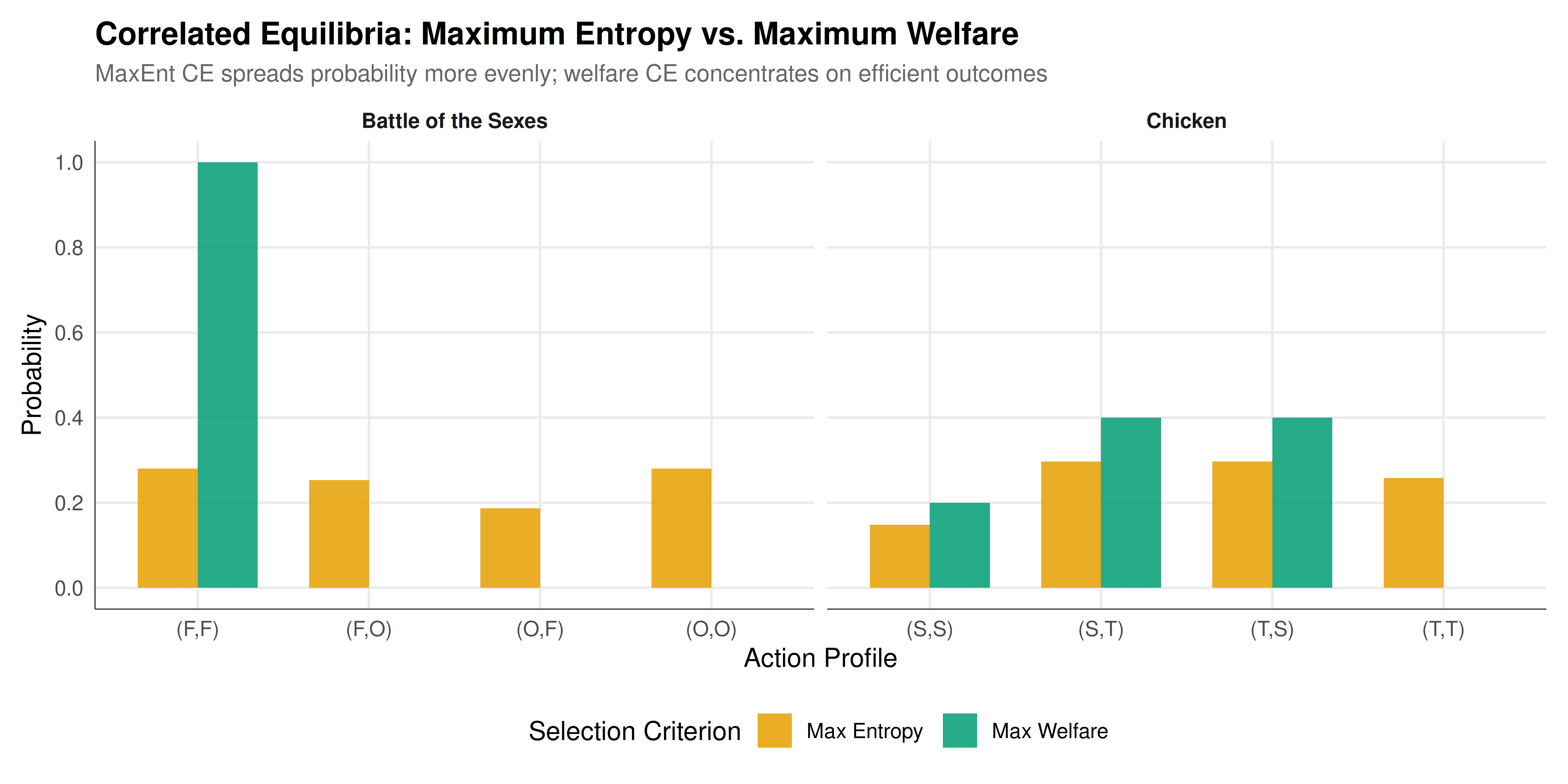
The figure compares the MaxEnt and welfare-maximising correlated equilibria across both games, showing the probability distributions as bar charts side by side.
```{r}
#| label: fig-maxent-ce-static
#| fig-cap: "Maximum-entropy and welfare-maximising correlated equilibria for Chicken and Battle of the Sexes. Entropy maximisation can assign probability to inefficient outcomes. The welfare solver returns one maximizing vertex; ties are not resolved by a secondary fairness or entropy criterion."
#| dev: [png, pdf]
#| fig-width: 10
#| fig-height: 5
#| dpi: 300
# Prepare data
ce_data <- data.frame(
  game = rep(c("Chicken", "Chicken", "Battle of the Sexes", "Battle of the Sexes"), each = 4),
  criterion = rep(c("Max Entropy", "Max Welfare", "Max Entropy", "Max Welfare"), each = 4),
  outcome = rep(c("(S,S)", "(S,T)", "(T,S)", "(T,T)"), 4),
  probability = c(
    as.numeric(maxent_chicken$p),
    as.numeric(welfare_chicken$p),
    as.numeric(maxent_bos$p),
    as.numeric(welfare_bos$p)
  )
)

# Relabel outcomes for BoS
ce_data$outcome[ce_data$game == "Battle of the Sexes"] <- rep(c("(O,O)", "(O,F)", "(F,O)", "(F,F)"), 2)

p_static <- ggplot(ce_data, aes(x = outcome, y = probability, fill = criterion)) +
  geom_col(position = "dodge", width = 0.7, alpha = 0.85) +
  facet_wrap(~ game, scales = "free_x", nrow = 1) +
  scale_fill_manual(
    values = c("Max Entropy" = okabe_ito[1], "Max Welfare" = okabe_ito[3]),
    name = "Selection Criterion"
  ) +
  scale_y_continuous(limits = c(0, 1), breaks = seq(0, 1, 0.2)) +
  labs(
    title = "Correlated Equilibria: Maximum Entropy vs. Maximum Welfare",
    subtitle = "MaxEnt CE spreads probability more evenly; welfare CE concentrates on efficient outcomes",
    x = "Action Profile", y = "Probability"
  ) +
  theme_publication() +
  theme(strip.text = element_text(face = "bold"))

p_static
```
## Interactive figure
The interactive version allows detailed inspection of each probability value and comparison across criteria.
```{r}
#| label: fig-maxent-ce-interactive
ce_data <- ce_data |>
  mutate(
    tooltip_text = paste0(
      "Game: ", game, "\n",
      "Criterion: ", criterion, "\n",
      "Outcome: ", outcome, "\n",
      "Probability: ", round(probability, 4)
    )
  )

p_inter <- ggplot(ce_data, aes(x = outcome, y = probability, fill = criterion,
                                text = tooltip_text)) +
  geom_col(position = "dodge", width = 0.7, alpha = 0.85) +
  facet_wrap(~ game, scales = "free_x", nrow = 1) +
  scale_fill_manual(
    values = c("Max Entropy" = okabe_ito[1], "Max Welfare" = okabe_ito[3]),
    name = "Criterion"
  ) +
  labs(
    title = "Correlated Equilibria (Interactive)",
    x = "Action Profile", y = "Probability"
  ) +
  theme_publication()

ggplotly(p_inter, tooltip = "text") |>
  config(displaylogo = FALSE, modeBarButtonsToRemove = c("select2d", "lasso2d"))
```
## Interpretation
Maximum entropy and maximum welfare are different selection criteria on the same CE polytope. Both distributions satisfy obedience constraints. Entropy has a unique maximizer in probability space; a linear welfare objective may have multiple maximizers. The code returns the first maximizing vertex, so its tie choice must not be interpreted as a fairness principle.
In Chicken, mutual swerve and the two asymmetric outcomes each have total payoff 6, while a crash has total payoff 0. Feasible welfare-maximizing equilibria can place weight on efficient profiles in more than one way. The maximum-entropy solution can retain positive crash probability because spreading probability raises entropy. The displayed distributions and computed welfare quantify that trade-off for these payoffs.
Mutual information measures dependence between the two action recommendations. It equals zero for every product-distribution Nash equilibrium, which is also a correlated equilibrium. Maximizing joint entropy does not generally minimize mutual information: the latter is the sum of marginal entropies minus joint entropy, and the marginals vary across the feasible set. In particular, a selected pure welfare-maximizing equilibrium has zero mutual information despite low joint entropy. Use the printed quantities rather than assuming an ordering between these criteria.
Maximum entropy is a well-defined selection rule under the stated incentive constraints, not a proof about how real players coordinate or about a mediator's minimum communication cost. Communication protocols, fairness preferences and information-design objectives require additional assumptions. This small base-R implementation enumerates vertices only for two-by-two games; larger games need a suitably qualified convex optimizer.
## Extensions & related tutorials
- [Entropy and strategic information](../../information-theory/entropy-and-strategic-information/) -- foundational information-theoretic concepts applied to games
- [Value of information in games](../../information-theory/value-of-information-games/) -- quantifying the strategic value of private information using entropy and mutual information
- [Cheap talk and communication](../../information-theory/cheap-talk-communication/) -- how costless messages can coordinate play and relate to correlation devices
- [LP duality and zero-sum games](../../linear-algebra-matrix/lp-duality-zero-sum/) -- linear programming methods for game-theoretic optimisation
- [Nash equilibrium original proof](../../history-of-gt-mathematics/nash-equilibrium-original-proof/) -- from independent randomisation (Nash) to correlated equilibrium (Aumann)
## References
::: {#refs}
:::