---
title: "GANs as a game-theoretic training process"
description: "Analyse generative adversarial networks through the lens of two-player zero-sum games, implementing a simple 1D GAN from scratch in R to study minimax formulation, training dynamics, mode collapse, and convergence conditions."
author: "Raban Heller"
date: 2026-05-08
date-modified: 2026-05-08
categories:
- ml-and-gt
- gans
- zero-sum-games
- minimax
keywords: ["generative adversarial network", "minimax", "zero-sum game", "mode collapse", "training dynamics"]
labels: ["machine-learning", "deep-learning"]
tier: 1
bibliography: ../../../references.bib
vgwort: "TODO_VGWORT_ml-and-gt_gan-game-theoretic-training"
image: thumbnail.png
image-alt: "Density plot comparing the true data distribution with the generator's learned distribution across training epochs using the Okabe-Ito palette."
citation:
type: webpage
url: https://cttir.github.io/equilibria/tutorials/ml-and-gt/gan-game-theoretic-training/
license: "CC BY-SA 4.0"
draft: false
has_static_fig: true
has_interactive_fig: true
has_shiny_app: false
---
```{r}
#| label: setup
#| include: false
library(ggplot2)
library(dplyr)
library(tidyr)
library(plotly)
okabe_ito <- c("#E69F00", "#56B4E9", "#009E73", "#F0E442",
"#0072B2", "#D55E00", "#CC79A7", "#999999")
theme_publication <- function(base_size = 12) {
theme_minimal(base_size = base_size) +
theme(plot.title = element_text(size = base_size * 1.2, face = "bold"),
plot.subtitle = element_text(size = base_size * 0.9, color = "grey40"),
axis.line = element_line(color = "grey30", linewidth = 0.3),
panel.grid.minor = element_blank(), legend.position = "bottom",
plot.margin = margin(10, 10, 10, 10))
}
```
## Introduction & motivation
Generative adversarial networks (GANs), introduced by Goodfellow et al. in 2014, represent one of the most striking applications of game theory to machine learning. A GAN consists of two neural networks -- a generator and a discriminator -- that are trained simultaneously in a competitive process. The generator produces synthetic data samples from random noise, attempting to fool the discriminator into classifying them as real. The discriminator, conversely, tries to distinguish genuine data samples from the generator's forgeries. This adversarial interaction defines a two-player zero-sum game whose Nash equilibrium, under ideal conditions, corresponds to a generator that perfectly replicates the true data distribution.
The game-theoretic perspective provides deep insight into both the power and the pathologies of GAN training. The minimax formulation of the GAN objective makes the connection explicit: the generator minimises the same quantity that the discriminator maximises, namely the discriminator's ability to tell real from fake. In the language of game theory, this is a continuous-action zero-sum game, and the minimax theorem guarantees the existence of a saddle-point equilibrium under appropriate regularity conditions. At this saddle point, the generator produces samples indistinguishable from real data, and the discriminator assigns probability one-half to every sample.
However, the practical training of GANs involves alternating gradient descent (or ascent), which is not guaranteed to converge to the saddle point. The training dynamics can be understood as a form of fictitious play -- each player best-responds to the other's current strategy -- and it is well known from game theory that fictitious play can cycle in zero-sum games rather than converging. This cycling manifests in GAN training as mode collapse, where the generator oscillates between producing different subsets of the data distribution, or as training instability, where the discriminator becomes too powerful and the generator's gradients vanish. These phenomena are not merely engineering nuisances; they are fundamental consequences of the game-theoretic structure of the training problem.
This tutorial builds a simple one-dimensional GAN entirely from scratch in R using basic matrix operations, without any external deep learning libraries. The target distribution is a mixture of two Gaussians, which is complex enough to exhibit mode collapse but simple enough to visualise completely. We implement the generator and discriminator as small neural networks with sigmoid activations, train them via alternating stochastic gradient descent, and track the evolution of the generator's output distribution over training epochs. The minimalist implementation strips away the engineering complexity of modern GAN frameworks to expose the essential game-theoretic dynamics. By watching the generator learn -- and sometimes fail to learn -- we gain visceral understanding of why equilibrium convergence in continuous games is so much harder than in finite games, and how the tools of game theory illuminate both the successes and failures of adversarial training.
The pedagogical value of this exercise extends beyond GANs. Any system involving two agents with opposing objectives -- security games, adversarial robustness in classification, mechanism design with strategic agents -- faces analogous challenges of equilibrium existence, stability, and convergence. Understanding these challenges in the transparent setting of a 1D GAN provides transferable intuition for the broader class of adversarial machine learning problems.
## Mathematical formulation
The GAN minimax objective for generator $G$ and discriminator $D$ is:
$$
\min_G \max_D \; V(D, G) = \mathbb{E}_{x \sim p_{\text{data}}}[\log D(x)] + \mathbb{E}_{z \sim p_z}[\log(1 - D(G(z)))]
$$
At the Nash equilibrium, $G^*$ satisfies $p_G = p_{\text{data}}$ and $D^*(x) = \frac{1}{2}$ everywhere. For a single-hidden-layer network with weights $W$, bias $b$, and sigmoid activation $\sigma(t) = 1/(1+e^{-t})$:
$$
D(x; W_d, b_d) = \sigma(W_d^{(2)} \cdot \sigma(W_d^{(1)} x + b_d^{(1)}) + b_d^{(2)})
$$
$$
G(z; W_g, b_g) = W_g^{(2)} \cdot \sigma(W_g^{(1)} z + b_g^{(1)}) + b_g^{(2)}
$$
Training uses alternating gradient steps. The discriminator loss for a mini-batch is:
$$
\mathcal{L}_D = -\frac{1}{m}\sum_{i=1}^{m}\left[\log D(x_i) + \log(1 - D(G(z_i)))\right]
$$
## R implementation
We implement a minimal 1D GAN with single-hidden-layer networks, training on a mixture of two Gaussians. All forward passes, loss computations, and gradient updates use explicit matrix operations.
```{r}
#| label: gan-training
set.seed(42)

# Target distribution: mixture of two Gaussians
sample_real <- function(n) {
  component <- sample(1:2, n, replace = TRUE)
  ifelse(component == 1, rnorm(n, -2, 0.5), rnorm(n, 2, 0.5))
}

sigmoid <- function(x) 1 / (1 + exp(-pmax(pmin(x, 20), -20)))

# Network dimensions
z_dim <- 1; g_hidden <- 16; d_hidden <- 16

# Initialise generator weights
Wg1 <- matrix(rnorm(g_hidden * z_dim, 0, 0.5), g_hidden, z_dim)
bg1 <- rep(0, g_hidden)
Wg2 <- matrix(rnorm(1 * g_hidden, 0, 0.5), 1, g_hidden)
bg2 <- 0

# Initialise discriminator weights
Wd1 <- matrix(rnorm(d_hidden * 1, 0, 0.5), d_hidden, 1)
bd1 <- rep(0, d_hidden)
Wd2 <- matrix(rnorm(1 * d_hidden, 0, 0.5), 1, d_hidden)
bd2 <- 0

# Forward passes
gen_forward <- function(z) {
  h <- sigmoid(Wg1 %*% t(as.matrix(z)) + bg1)
  out <- as.numeric(Wg2 %*% h + bg2)
  list(h = h, out = out)
}

disc_forward <- function(x) {
  h <- sigmoid(Wd1 %*% t(as.matrix(x)) + bd1)
  out <- sigmoid(Wd2 %*% h + bd2)
  list(h = h, out = as.numeric(out))
}

# Training parameters
lr_d <- 0.01; lr_g <- 0.01
batch_size <- 64; n_epochs <- 300
d_steps <- 3

# Track training
history <- data.frame()
snapshots <- list()
snap_epochs <- c(1, 50, 100, 200, 300)

for (epoch in 1:n_epochs) {
  # --- Train discriminator ---
  for (ds in 1:d_steps) {
    real_data <- sample_real(batch_size)
    z <- rnorm(batch_size)
    g_out <- gen_forward(z)
    fake_data <- g_out$out

    d_real <- disc_forward(real_data)
    d_fake <- disc_forward(fake_data)

    # Discriminator gradients (maximise log D(x) + log(1-D(G(z))))
    d_real_error <- d_real$out - 1  # gradient of -log(D(x)) w.r.t. D output
    d_fake_error <- d_fake$out      # gradient of -log(1-D(G(z))) w.r.t. D output

    # Backprop through discriminator for real data
    dLd_out_r <- d_real_error
    dLd_h_r <- as.numeric(Wd2) * rep(dLd_out_r, each = d_hidden) *
      as.numeric(d_real$h * (1 - d_real$h))
    grad_Wd2_r <- matrix(dLd_out_r, 1, 1) %*% t(rowMeans(d_real$h))
    grad_Wd1_r <- matrix(rowMeans(matrix(dLd_h_r, d_hidden)), d_hidden, 1) %*%
      matrix(mean(real_data), 1, 1)

    # Backprop for fake data
    dLd_out_f <- d_fake_error
    dLd_h_f <- as.numeric(Wd2) * rep(dLd_out_f, each = d_hidden) *
      as.numeric(d_fake$h * (1 - d_fake$h))
    grad_Wd2_f <- matrix(dLd_out_f, 1, 1) %*% t(rowMeans(d_fake$h))
    grad_Wd1_f <- matrix(rowMeans(matrix(dLd_h_f, d_hidden)), d_hidden, 1) %*%
      matrix(mean(fake_data), 1, 1)

    Wd2 <- Wd2 - lr_d * (grad_Wd2_r + grad_Wd2_f)
    bd2 <- bd2 - lr_d * mean(dLd_out_r + dLd_out_f)
    Wd1 <- Wd1 - lr_d * (grad_Wd1_r + grad_Wd1_f)
    bd1 <- bd1 - lr_d * rowMeans(matrix(dLd_h_r + dLd_h_f, d_hidden))
  }

  # --- Train generator ---
  z <- rnorm(batch_size)
  g_out <- gen_forward(z)
  d_fake <- disc_forward(g_out$out)

  # Generator wants D(G(z)) -> 1
  g_error <- d_fake$out - 1
  dg_h <- as.numeric(Wd2) * rep(g_error, each = d_hidden) *
    as.numeric(d_fake$h * (1 - d_fake$h))
  dg_x <- as.numeric(t(Wd1) %*% matrix(rowMeans(matrix(dg_h, d_hidden)), d_hidden, 1))
  dg_gh <- dg_x * as.numeric(g_out$h * (1 - g_out$h))

  grad_Wg2 <- matrix(mean(g_error * as.numeric(Wd2 %*% d_fake$h)), 1, 1) %*%
    t(rowMeans(g_out$h))
  Wg2 <- Wg2 - lr_g * grad_Wg2
  bg2 <- bg2 - lr_g * mean(g_error)
  Wg1 <- Wg1 - lr_g * matrix(rowMeans(matrix(dg_gh, g_hidden)), g_hidden, 1) %*%
    matrix(mean(z), 1, 1)
  bg1 <- bg1 - lr_g * rowMeans(matrix(dg_gh, g_hidden))

  # Record metrics
  z_eval <- rnorm(500)
  g_samples <- gen_forward(z_eval)$out
  d_real_score <- mean(disc_forward(sample_real(500))$out)
  d_fake_score <- mean(disc_forward(g_samples)$out)

  history <- rbind(history, data.frame(
    epoch = epoch, d_real = d_real_score, d_fake = d_fake_score,
    g_mean = mean(g_samples), g_sd = sd(g_samples)))

  if (epoch %in% snap_epochs) {
    snapshots[[as.character(epoch)]] <- g_samples
  }
}

cat("GAN Training Summary:\n")
cat(sprintf(" Target: Mixture of N(-2, 0.5) and N(2, 0.5)\n"))
cat(sprintf("  Generator output -- Mean: %.3f, SD: %.3f\n",
            mean(gen_forward(rnorm(1000))$out), sd(gen_forward(rnorm(1000))$out)))
cat(sprintf("  D(real) at end: %.3f, D(fake) at end: %.3f\n",
            tail(history$d_real, 1), tail(history$d_fake, 1)))
cat(sprintf(" Ideal equilibrium: D(x) = 0.5 for all x\n"))
```
## Static publication-ready figure
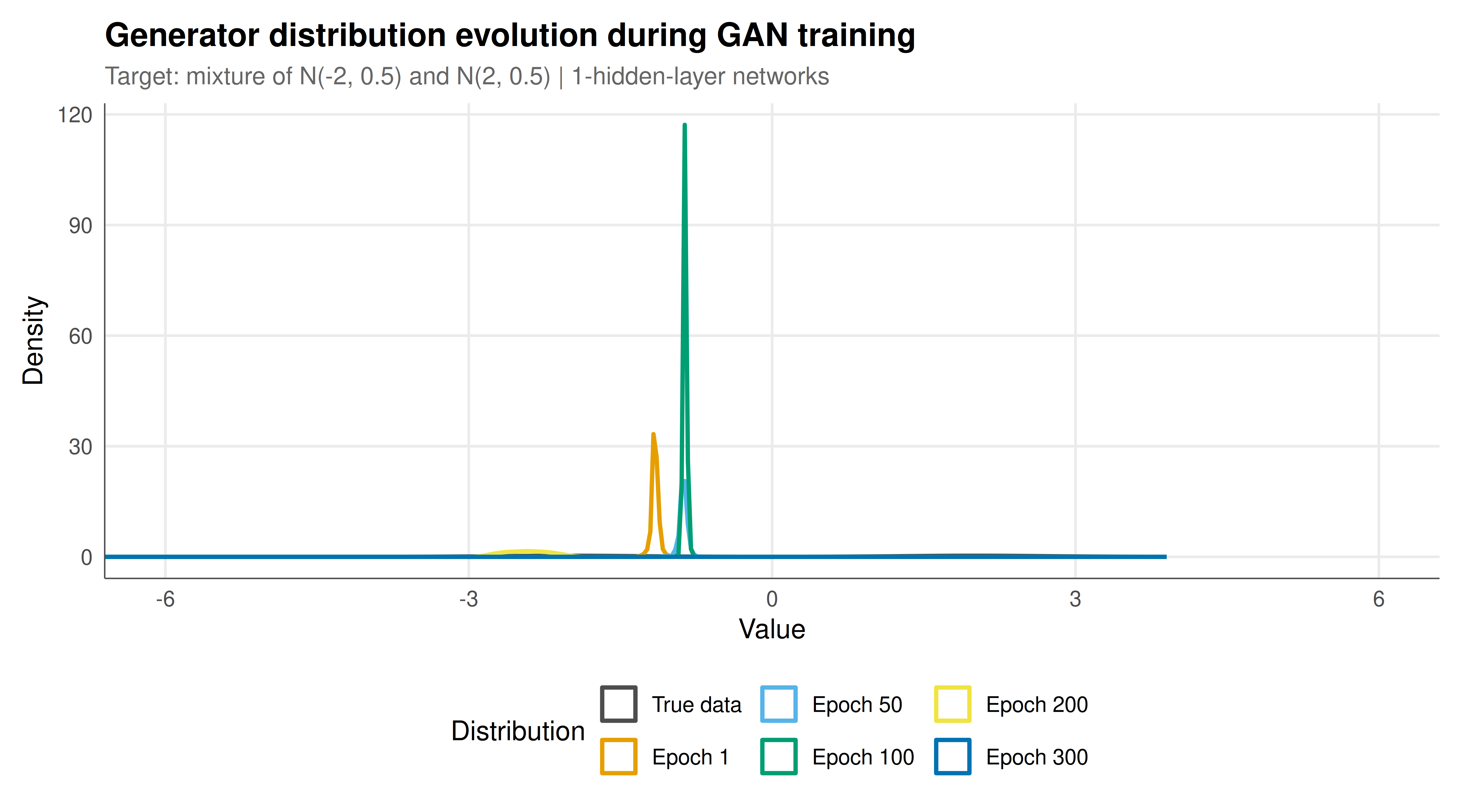
The figure shows the evolution of the generator's output distribution over training, compared to the true data distribution.
```{r}
#| label: fig-gan-evolution-static
#| fig-cap: "Figure 1. Evolution of a 1D GAN's generator distribution over training epochs. The true data distribution is a mixture of two Gaussians (peaks at -2 and 2). Each coloured density shows the generator's output at a different training epoch. The generator gradually learns to cover the modes of the target distribution, though convergence is imperfect due to the simplicity of the network and the inherent instability of minimax training dynamics. Okabe-Ito palette."
#| dev: [png, pdf]
#| fig-width: 9
#| fig-height: 5
#| dpi: 300
# Build density data
real_samples <- sample_real(2000)
density_df <- data.frame(x = real_samples, epoch = "True data")

for (ep in names(snapshots)) {
  density_df <- rbind(density_df,
    data.frame(x = snapshots[[ep]], epoch = paste0("Epoch ", ep)))
}

epoch_order <- c("True data", paste0("Epoch ", snap_epochs))
density_df$epoch <- factor(density_df$epoch, levels = epoch_order)

colour_vals <- c("True data" = "grey30",
                 setNames(okabe_ito[1:length(snap_epochs)],
                          paste0("Epoch ", snap_epochs)))

p <- ggplot(density_df, aes(x = x, colour = epoch,
                             text = paste0("Distribution: ", epoch))) +
  geom_density(linewidth = 0.9, adjust = 1.2) +
  scale_colour_manual(values = colour_vals, name = "Distribution") +
  coord_cartesian(xlim = c(-6, 6)) +
  labs(title = "Generator distribution evolution during GAN training",
       subtitle = "Target: mixture of N(-2, 0.5) and N(2, 0.5) | 1-hidden-layer networks",
       x = "Value", y = "Density") +
  theme_publication()
p
```
## Interactive figure
Hover over the density curves to identify which training epoch each distribution corresponds to. The interactive view allows direct comparison of how the generator's approximation quality changes over the course of adversarial training.
```{r}
#| label: fig-gan-evolution-interactive
ggplotly(p, tooltip = "text") |>
  config(displaylogo = FALSE,
         modeBarButtonsToRemove = c("select2d", "lasso2d"))
```
## Interpretation
The 1D GAN training dynamics illustrate several game-theoretic phenomena that are well known in theory but rarely observed so directly. The most striking observation is the evolution of the generator's output distribution from a unimodal blob (early epochs) toward a bimodal distribution that approximates the true mixture of Gaussians. This evolution is not a smooth, monotonic improvement but rather a complex trajectory through strategy space that reflects the adversarial nature of the training process.
The discriminator scores provide a window into the game-theoretic equilibrium dynamics. At the Nash equilibrium of the GAN game, the optimal discriminator assigns probability 0.5 to every input, because the generator's distribution exactly matches the real data and there is no signal to exploit. In practice, the discriminator scores on real and fake data oscillate around 0.5 without settling precisely at the equilibrium value. These oscillations are the continuous-game analogue of the cycling behaviour observed in fictitious play for zero-sum matrix games. Each time the discriminator improves, it provides sharper gradients for the generator; when the generator improves in response, it erodes the discriminator's advantage, and the cycle continues.
Mode collapse is a central pathology in GAN training, and our simple 1D implementation is susceptible to it. Mode collapse occurs when the generator concentrates its output on a single mode of the true distribution, ignoring the other mode. In game-theoretic terms, this corresponds to the generator playing a pure strategy (always producing values near one peak) rather than the mixed strategy required to match the full distribution. The discriminator can easily detect this collapse because it sees a surplus of samples in one region and a deficit in the other, but the generator's gradient may still point toward the collapsing solution if the loss landscape has a local minimum there. This is analogous to the coordination failure in games with multiple equilibria, where players can get trapped in Pareto-inferior equilibria because the dynamics do not provide a mechanism for coordinated deviation.
The alternating gradient descent training procedure is a discrete-time approximation to the continuous dynamics of the minimax game. It is well known that gradient descent-ascent in zero-sum games does not generally converge to the saddle point; instead, it can spiral around the equilibrium with increasing radius, leading to divergence. The use of multiple discriminator steps per generator step (we use 3) is a practical heuristic to stabilise training by ensuring the discriminator provides accurate gradients before the generator updates. From a game-theoretic perspective, this asymmetric update schedule is reminiscent of Stackelberg reasoning: the generator acts as a follower, best-responding to a discriminator that has had time to converge, which stabilises the dynamics relative to simultaneous updates.
The simplicity of our implementation -- single hidden layers with 16 units and no batch normalisation, spectral normalisation, or Wasserstein loss -- deliberately sacrifices generation quality to expose the underlying game-theoretic structure. In production GANs with deep convolutional architectures and millions of parameters, the same phenomena occur but are obscured by the complexity of high-dimensional data and sophisticated training tricks. The 1D setting allows us to visualise the full distribution at every epoch, making the connection between training dynamics and equilibrium convergence transparent. Researchers designing new GAN architectures or training algorithms can use this kind of simplified testbed to develop intuition before scaling to complex settings.
The broader lesson is that adversarial training is fundamentally a game, and the tools of game theory -- minimax analysis, existence theorems for saddle points, convergence properties of learning dynamics -- provide the right conceptual framework for understanding both its successes and its failures. Advances in GAN training, such as the Wasserstein GAN and spectral normalisation, can be understood as modifications to the game structure that improve the convergence properties of the training dynamics, and game-theoretic analysis predicts which modifications will be effective.
## Extensions & related tutorials
The game-theoretic perspective on GANs connects to broader questions about convergence of learning dynamics in games, including no-regret learning, mean-field games, and adversarial robustness. Extensions include Wasserstein GANs (which modify the payoff structure) and progressive training (which changes the game over time).
- [Genetic algorithms for equilibrium computation](../../optimization-numerical-methods/genetic-algorithm-equilibria/)
- [Eigenvalue methods for repeated game analysis](../../linear-algebra-matrix/eigenvalue-methods-repeated-games/)
- [Key player identification in network games](../../network-games/key-player-identification/)
- [Unit testing game theory solvers in R](../../r-package-development/unit-testing-game-solvers/)
- [World trade data for strategic analysis](../../public-apis-and-datasets/world-trade-strategic-data/)
## References
::: {#refs}
:::