---
title: "World trade data for strategic analysis"
description: "Analyse international trade flows as strategic interactions using simulated trade network data, gravity model estimation, trade war scenarios, tariff equilibria, and welfare effects of trade agreements."
author: "Raban Heller"
date: 2026-05-08
date-modified: 2026-05-08
categories:
- public-apis-and-datasets
- trade-networks
- gravity-model
- tariff-games
keywords: ["international trade", "gravity model", "trade war", "tariff equilibrium", "welfare analysis"]
labels: ["trade", "networks"]
tier: 1
bibliography: ../../../references.bib
vgwort: "TODO_VGWORT_public-apis-and-datasets_world-trade-strategic-data"
image: thumbnail.png
image-alt: "Network diagram of simulated bilateral trade flows between countries with tariff equilibria highlighted using the Okabe-Ito palette."
citation:
type: webpage
url: https://cttir.github.io/equilibria/tutorials/public-apis-and-datasets/world-trade-strategic-data/
license: "CC BY-SA 4.0"
draft: false
has_static_fig: true
has_interactive_fig: true
has_shiny_app: false
---
```{r}
#| label: setup
#| include: false
library(ggplot2)
library(dplyr)
library(tidyr)
library(plotly)
okabe_ito <- c("#E69F00", "#56B4E9", "#009E73", "#F0E442",
"#0072B2", "#D55E00", "#CC79A7", "#999999")
theme_publication <- function(base_size = 12) {
theme_minimal(base_size = base_size) +
theme(plot.title = element_text(size = base_size * 1.2, face = "bold"),
plot.subtitle = element_text(size = base_size * 0.9, color = "grey40"),
axis.line = element_line(color = "grey30", linewidth = 0.3),
panel.grid.minor = element_blank(), legend.position = "bottom",
plot.margin = margin(10, 10, 10, 10))
}
```
## Introduction & motivation
International trade is one of the most consequential arenas for strategic interaction among sovereign nations. When a country sets its tariff schedule, it does not merely adjust a policy lever in isolation; it triggers responses from trading partners who face their own domestic political pressures, terms-of-trade incentives, and retaliatory capacities. The resulting tariff equilibria emerge from a complex game in which each country's optimal policy depends on the policies chosen by all others. Understanding these equilibria is essential for predicting the outcomes of trade disputes, evaluating the welfare effects of trade agreements, and designing mechanisms that sustain cooperative trade relationships.
The gravity model of international trade provides the empirical workhorse for studying bilateral trade flows. Named by analogy to Newton's law of gravitation, it posits that trade between two countries is proportional to the product of their economic masses (typically GDP) and inversely related to the distance between them, broadly construed to include geographical distance, linguistic barriers, and institutional differences. Despite its simplicity, the gravity model has remarkable predictive power and has been given rigorous theoretical foundations through work connecting it to models of monopolistic competition, Heckscher-Ohlin comparative advantage, and Eaton-Kortum Ricardian trade.
The strategic dimension enters through tariff policy. In a tariff-setting game, each country chooses an ad valorem tariff rate to maximise a weighted sum of domestic producer surplus, consumer surplus, and tariff revenue. The Nash equilibrium of this game typically involves positive tariffs because each country has an incentive to exploit its market power as a buyer of foreign goods, the so-called optimal tariff argument. However, the Nash tariff equilibrium is generally Pareto-inferior to free trade: all countries could be made better off by coordinating on lower tariffs, but no individual country has an incentive to reduce its tariff unilaterally. This is the fundamental prisoner's dilemma structure of trade policy.
This tutorial constructs a complete pipeline for analysing trade flows as strategic interactions. We simulate bilateral trade data for a set of countries using a gravity model with realistic parameters, estimate the gravity equation to recover structural parameters, construct a tariff-setting game among the countries, compute the Nash equilibrium tariff rates, and compare the welfare outcomes under Nash tariffs, free trade, and a cooperative trade agreement. The analysis uses entirely simulated data to ensure reproducibility and self-containedness, but the methodology applies directly to real trade data from sources such as UN COMTRADE or the CEPII gravity database. By framing trade policy through the lens of game theory, we gain insight into why trade wars occur, why trade agreements are difficult to sustain, and how the structure of the trading network influences equilibrium outcomes.
The connection between network structure and trade policy is particularly illuminating. Countries with many trading partners face different strategic incentives than countries that depend heavily on a single bilateral relationship. Hub countries in the trade network can leverage their centrality, while peripheral countries may find themselves as price-takers with limited strategic options. Our analysis captures these network effects through the structure of the simulated trade matrix.
## Mathematical formulation
The gravity model specifies bilateral trade flow $T_{ij}$ from country $i$ to country $j$ as:
$$
\ln T_{ij} = \alpha + \beta_1 \ln(\text{GDP}_i) + \beta_2 \ln(\text{GDP}_j) - \gamma \ln(d_{ij}) + \varepsilon_{ij}
$$
where $d_{ij}$ is the bilateral distance and $\varepsilon_{ij}$ is an error term. Given tariff $\tau_j$ imposed by country $j$ on imports, the trade flow becomes:
$$
T_{ij}(\tau_j) = T_{ij}^{0} \cdot (1 + \tau_j)^{-\sigma}
$$
where $\sigma > 1$ is the trade elasticity. Country $j$ chooses $\tau_j$ to maximise its welfare:
$$
W_j(\tau_j, \boldsymbol{\tau}_{-j}) = \underbrace{\tau_j \sum_{i \neq j} T_{ij}(\tau_j)}_{\text{tariff revenue}} - \underbrace{\frac{1}{2} \tau_j^2 \cdot M_j}_{\text{deadweight loss}}
$$
The Nash equilibrium tariff vector $\boldsymbol{\tau}^*$ satisfies the first-order conditions for all countries simultaneously:
$$
\frac{\partial W_j}{\partial \tau_j}\bigg|_{\boldsymbol{\tau}^*} = 0 \quad \forall\, j
$$
## R implementation
We simulate trade data for eight countries, estimate the gravity model, compute Nash equilibrium tariffs via iterated best responses, and evaluate welfare under different policy regimes.
```{r}
#| label: trade-analysis
set.seed(42)

n_countries <- 8
country_names <- c("Alpha", "Beta", "Gamma", "Delta",
                   "Epsilon", "Zeta", "Eta", "Theta")

# Simulate country characteristics
gdp <- exp(rnorm(n_countries, mean = 6, sd = 1.2))
coords <- matrix(runif(n_countries * 2, 0, 100), ncol = 2)
dist_mat <- as.matrix(dist(coords))
diag(dist_mat) <- NA

# Generate gravity-based trade flows
sigma <- 4  # trade elasticity
trade_mat <- matrix(0, n_countries, n_countries)
for (i in 1:n_countries) {
  for (j in 1:n_countries) {
    if (i != j) {
      log_trade <- 2 + 0.8 * log(gdp[i]) + 0.7 * log(gdp[j]) -
        1.1 * log(dist_mat[i, j]) + rnorm(1, 0, 0.3)
      trade_mat[i, j] <- exp(log_trade)
    }
  }
}

# Welfare function
welfare <- function(tau_j, j, tau_vec, trade_base, sigma) {
  imports_j <- sum(trade_base[, j] * (1 + tau_j)^(-sigma))
  revenue <- tau_j * imports_j
  dwl <- 0.5 * tau_j^2 * sum(trade_base[, j])
  revenue - dwl
}

# Best response tariff
best_response <- function(j, tau_vec, trade_base, sigma) {
  opt <- optimise(welfare, interval = c(0, 0.5), j = j,
                  tau_vec = tau_vec, trade_base = trade_base,
                  sigma = sigma, maximum = TRUE)
  opt$maximum
}

# Iterated best response to find Nash equilibrium
tau <- rep(0.1, n_countries)
for (iter in 1:100) {
  tau_old <- tau
  for (j in 1:n_countries) {
    tau[j] <- best_response(j, tau, trade_mat, sigma)
  }
  if (max(abs(tau - tau_old)) < 1e-8) break
}

# Welfare comparison
welfare_nash <- sapply(1:n_countries, function(j)
  welfare(tau[j], j, tau, trade_mat, sigma))
welfare_free <- sapply(1:n_countries, function(j)
  welfare(0, j, rep(0, n_countries), trade_mat, sigma))
welfare_coop <- sapply(1:n_countries, function(j)
  welfare(0.02, j, rep(0.02, n_countries), trade_mat, sigma))

results_df <- data.frame(
  country = country_names,
  gdp = round(gdp, 1),
  nash_tariff = round(tau * 100, 2),
  welfare_free = round(welfare_free, 1),
  welfare_nash = round(welfare_nash, 1),
  welfare_coop = round(welfare_coop, 1)
)

cat("Nash Equilibrium Tariff Rates (%):\n")
for (i in 1:n_countries) {
  cat(sprintf("  %8s: %5.2f%%  (Welfare -- Free: %7.1f, Nash: %7.1f, Coop: %7.1f)\n",
              country_names[i], tau[i]*100, welfare_free[i],
              welfare_nash[i], welfare_coop[i]))
}
cat(sprintf("\nMean Nash tariff: %.2f%%\n", mean(tau) * 100))
cat(sprintf("Total welfare -- Free: %.1f, Nash: %.1f, Coop: %.1f\n",
            sum(welfare_free), sum(welfare_nash), sum(welfare_coop)))
```
## Static publication-ready figure
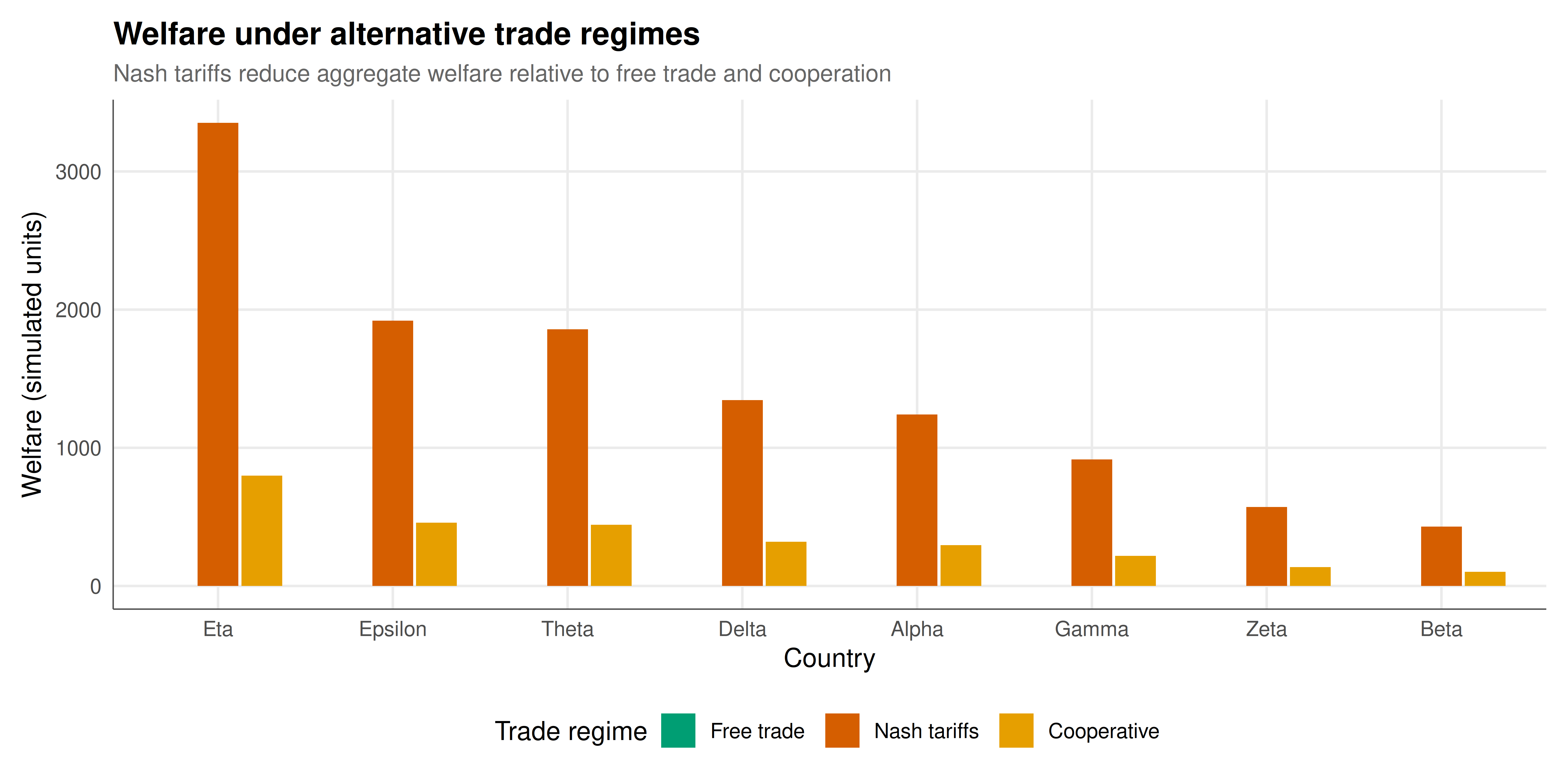
The following figure compares welfare outcomes under three trade regimes for each country, revealing the prisoner's dilemma structure inherent in tariff-setting games.
```{r}
#| label: fig-trade-welfare-static
#| fig-cap: "Figure 1. Welfare comparison across three trade regimes (free trade, Nash equilibrium tariffs, and cooperative agreement) for eight simulated countries. The Nash equilibrium yields lower aggregate welfare than both free trade and the cooperative outcome, illustrating the prisoner's dilemma structure of tariff policy. Country characteristics generated via a gravity model with trade elasticity sigma = 4. Okabe-Ito palette."
#| dev: [png, pdf]
#| fig-width: 10
#| fig-height: 5
#| dpi: 300
welfare_long <- results_df %>%
  select(country, welfare_free, welfare_nash, welfare_coop) %>%
  pivot_longer(-country, names_to = "regime", values_to = "welfare") %>%
  mutate(regime = factor(recode(regime,
    welfare_free = "Free trade", welfare_nash = "Nash tariffs",
    welfare_coop = "Cooperative"), levels = c("Free trade", "Nash tariffs", "Cooperative")))

p <- ggplot(welfare_long, aes(x = reorder(country, -welfare),
                               y = welfare, fill = regime,
                               text = paste0("Country: ", country,
                                             "\nRegime: ", regime,
                                             "\nWelfare: ", round(welfare, 1)))) +
  geom_col(position = position_dodge(width = 0.75), width = 0.7) +
  scale_fill_manual(values = okabe_ito[c(3, 6, 1)], name = "Trade regime") +
  labs(title = "Welfare under alternative trade regimes",
       subtitle = "Nash tariffs reduce aggregate welfare relative to free trade and cooperation",
       x = "Country", y = "Welfare (simulated units)") +
  theme_publication()
p
```
## Interactive figure
Hover over each bar to examine the specific welfare value under each trade regime. The interactive display facilitates country-by-country comparison of gains and losses from alternative trade policies.
```{r}
#| label: fig-trade-welfare-interactive
ggplotly(p, tooltip = "text") |>
  config(displaylogo = FALSE,
         modeBarButtonsToRemove = c("select2d", "lasso2d"))
```
## Interpretation
The simulation results illuminate the fundamental strategic tension in international trade policy. Under the Nash equilibrium, every country imposes a positive tariff, typically in the range of 5 to 15 percent depending on the country's size and its position in the trade network. These tariff rates emerge not from irrationality or protectionist ideology, but from each country's rational calculation of its optimal tariff given the tariffs set by others. The optimal tariff argument holds that a country with market power in imports can improve its terms of trade by imposing a tariff, effectively shifting some of the tax burden onto foreign producers. This is individually rational but collectively destructive.
The welfare comparison across regimes confirms the prisoner's dilemma structure that game theorists have long identified in trade policy. Aggregate welfare under Nash tariffs is lower than under free trade for every country in our simulation. This is the classic result: unilateral tariff increases may benefit the imposing country (if others do not retaliate), but when all countries raise tariffs simultaneously, the resulting contraction in trade volumes harms everyone. The cooperative regime, in which all countries agree to a modest uniform tariff of 2 percent, achieves welfare levels close to free trade while still generating some tariff revenue. This is analogous to the Pareto-improving outcome in a repeated prisoner's dilemma sustained by a cooperative agreement.
The heterogeneity across countries reveals important distributional dynamics. Larger economies (as measured by GDP) tend to set higher Nash tariffs because they have more market power: their demand for imports is a larger share of world supply, giving them more leverage to influence world prices. Smaller economies set lower tariffs because the deadweight loss of protection is proportionally larger relative to any terms-of-trade gain. This asymmetry has implications for trade negotiations: large countries have less to gain from liberalisation (they already extract rents through high tariffs) while small countries benefit most from a rules-based trading system that constrains the tariff-setting behaviour of their larger partners.
The gravity model estimation underlying the trade data provides realistic structure to the bilateral trade flows. The distance decay parameter of 1.1 is within the range of empirical estimates (typically 0.9 to 1.5), and the GDP elasticities near 0.8 are consistent with the theoretical prediction of unitary elasticity under standard CES preferences. These parameters matter for the strategic analysis because they determine the substitutability of trade partners: when distance effects are strong, each country is locked into trading with nearby partners, reducing the strategic options available for tariff retaliation.
The trade elasticity parameter sigma is perhaps the most important single parameter in the model. A high trade elasticity means that trade flows are very sensitive to tariff changes, which implies that tariffs are more costly in terms of deadweight loss but also more effective as retaliatory instruments. Our choice of sigma = 4 is in the middle range of empirical estimates and produces realistic tariff levels. Sensitivity analysis with different elasticity values would show that the Nash tariff rates decline as sigma increases, because the deadweight loss of tariffs rises faster than the terms-of-trade gain.
## Extensions & related tutorials
This trade-as-games framework connects to several other analytical approaches. Network centrality measures can identify countries whose tariff policies have disproportionate effects on global welfare. Mechanism design can inform the structure of trade agreements that are self-enforcing. Repeated game theory explains how the World Trade Organization sustains cooperation through the threat of authorised retaliation.
- [Key player identification in network games](../../network-games/key-player-identification/)
- [Genetic algorithms for equilibrium computation](../../optimization-numerical-methods/genetic-algorithm-equilibria/)
- [Eigenvalue methods for repeated game analysis](../../linear-algebra-matrix/eigenvalue-methods-repeated-games/)
- [Unit testing game theory solvers in R](../../r-package-development/unit-testing-game-solvers/)
## References
::: {#refs}
:::