---
title: "Key player identification in network games"
description: "Identify the most influential players in network games using Ballester-Calvo-Zenou intercentrality, analysing network effects on equilibrium play, optimal targeting policies, and applications to crime and R&D networks."
author: "Raban Heller"
date: 2026-05-08
date-modified: 2026-05-08
categories:
- network-games
- centrality
- key-player
- strategic-complements
keywords: ["network games", "Bonacich centrality", "intercentrality", "key player", "strategic interaction"]
labels: ["networks", "policy"]
tier: 1
bibliography: ../../../references.bib
vgwort: "TODO_VGWORT_network-games_key-player-identification"
image: thumbnail.png
image-alt: "Network graph with nodes sized by intercentrality and coloured by equilibrium action level using the Okabe-Ito palette."
citation:
type: webpage
url: https://cttir.github.io/equilibria/tutorials/network-games/key-player-identification/
license: "CC BY-SA 4.0"
draft: false
has_static_fig: true
has_interactive_fig: true
has_shiny_app: false
---
```{r}
#| label: setup
#| include: false
library(ggplot2)
library(dplyr)
library(tidyr)
library(plotly)
okabe_ito <- c("#E69F00", "#56B4E9", "#009E73", "#F0E442",
"#0072B2", "#D55E00", "#CC79A7", "#999999")
theme_publication <- function(base_size = 12) {
theme_minimal(base_size = base_size) +
theme(plot.title = element_text(size = base_size * 1.2, face = "bold"),
plot.subtitle = element_text(size = base_size * 0.9, color = "grey40"),
axis.line = element_line(color = "grey30", linewidth = 0.3),
panel.grid.minor = element_blank(), legend.position = "bottom",
plot.margin = margin(10, 10, 10, 10))
}
```
## Introduction & motivation
In many strategic environments, the interaction structure between players is not uniform but shaped by an underlying network. Criminals influence their immediate associates, firms share knowledge with research partners, students affect the study habits of their friends, and countries trade primarily with geographic neighbours. When strategic interactions are mediated by a network, the identity and position of individual players within that network become crucial determinants of aggregate outcomes. Removing a well-connected criminal from a network may reduce total crime far more than removing a peripheral one, even if both individuals have identical intrinsic propensities for criminal activity. The key player problem asks: which player's removal causes the largest reduction in aggregate equilibrium activity?
This question was formalised in the landmark work of Ballester, Calvo-Armengol, and Zenou (2006), who analysed a linear-quadratic network game in which each player's optimal action depends positively on the actions of their network neighbours (strategic complements). They showed that the Nash equilibrium of this game has a closed-form solution in terms of the Bonacich centrality of each player in the network, and that the key player -- the one whose removal reduces total equilibrium activity the most -- is identified by a new centrality measure they called intercentrality. Crucially, the key player is not necessarily the player with the highest Bonacich centrality or the highest degree. Intercentrality accounts for how a player's removal restructures the entire network, changing the equilibrium behaviour of all remaining players through cascading network effects.
The practical implications span criminal justice policy, public health interventions, research and development policy, and counter-terrorism strategy. In criminal networks, law enforcement faces a resource constraint: they can investigate and prosecute only a limited number of individuals. The key player analysis provides a principled criterion for targeting, one grounded in equilibrium reasoning rather than simple heuristics like targeting the most connected individual. In R&D networks, a government seeking to maximise innovation output might subsidise the key player -- the firm whose increased effort generates the largest positive spillovers throughout the network. In epidemiology, network games model vaccination decisions where each individual's incentive to vaccinate depends on the vaccination rates of their contacts.
This tutorial implements the full Ballester-Calvo-Zenou framework from scratch. We construct a random network, compute the Nash equilibrium of the linear-quadratic game in terms of Bonacich centrality, calculate the intercentrality of each player, identify the key player, and visualise how the equilibrium shifts when the key player is removed. The analysis highlights a recurring theme in network economics: local connectivity patterns aggregate into global equilibrium outcomes in non-obvious ways, and effective policy requires understanding these emergent structures rather than relying on intuition about individual-level characteristics.
The methodology extends beyond the linear-quadratic setting. While the closed-form Bonacich solution relies on linearity, the key player concept applies to any network game with strategic complements or substitutes. For nonlinear games, the key player can be identified numerically by computing equilibria with and without each player and comparing aggregate outcomes.
## Mathematical formulation
Consider $n$ players on a network with adjacency matrix $G$ (symmetric, zero diagonal). Player $i$ chooses action $x_i \geq 0$ to maximise:
$$
u_i(x_i, \mathbf{x}_{-i}) = \alpha_i x_i - \frac{1}{2} x_i^2 + \lambda \sum_{j=1}^{n} g_{ij} x_i x_j
$$
where $\alpha_i > 0$ is the standalone marginal benefit, $\lambda > 0$ captures the strength of strategic complementarities, and $g_{ij} \in \{0, 1\}$ indicates a link. The Nash equilibrium satisfies the first-order condition $x_i^* = \alpha_i + \lambda \sum_j g_{ij} x_j^*$, yielding in matrix form:
$$
\mathbf{x}^* = (I - \lambda G)^{-1} \boldsymbol{\alpha} = \mathbf{b}(G, \lambda, \boldsymbol{\alpha})
$$
where $\mathbf{b}(G, \lambda, \boldsymbol{\alpha})$ is the Bonacich centrality vector, valid when $\lambda < 1/\rho(G)$ with $\rho(G)$ the spectral radius of $G$. The intercentrality of player $i$ is defined as:
$$
c_i(G, \lambda) = \frac{b_i(G, \lambda, \boldsymbol{\alpha})^2}{m_{ii}(G, \lambda)}
$$
where $m_{ii} = [(I - \lambda G)^{-1}]_{ii}$. The key player is $i^* = \arg\max_i \; c_i(G, \lambda)$.
## R implementation
We simulate a network, compute Bonacich centrality, intercentrality, and identify the key player whose removal maximises the drop in aggregate equilibrium action.
```{r}
#| label: key-player-analysis
set.seed(42)

n <- 15  # number of players
# Generate random network (Erdos-Renyi)
prob_link <- 0.3
G <- matrix(0, n, n)
for (i in 1:(n-1)) {
  for (j in (i+1):n) {
    if (runif(1) < prob_link) { G[i,j] <- 1; G[j,i] <- 1 }
  }
}

# Ensure connected: add links to isolated nodes
degrees <- rowSums(G)
for (i in which(degrees == 0)) {
  j <- sample(setdiff(1:n, i), 1)
  G[i,j] <- 1; G[j,i] <- 1
}

# Parameters
alpha <- rep(1, n)  # homogeneous standalone benefits
spectral_radius <- max(eigen(G, only.values = TRUE)$values)
lambda <- 0.8 / spectral_radius  # ensure interior solution

# Bonacich centrality = Nash equilibrium actions
I_n <- diag(n)
M <- solve(I_n - lambda * G)
bonacich <- as.numeric(M %*% alpha)

# Intercentrality
m_diag <- diag(M)
intercentrality <- bonacich^2 / m_diag

# Key player identification
key_player <- which.max(intercentrality)

# Compute equilibrium without key player
G_reduced <- G[-key_player, -key_player]
alpha_reduced <- alpha[-key_player]
M_reduced <- solve(diag(n-1) - lambda * G_reduced)
bonacich_reduced <- as.numeric(M_reduced %*% alpha_reduced)

total_activity_full <- sum(bonacich)
total_activity_reduced <- sum(bonacich_reduced)
reduction <- total_activity_full - total_activity_reduced

# Build results data frame
player_df <- data.frame(
  player = 1:n,
  degree = rowSums(G),
  bonacich = round(bonacich, 4),
  intercentrality = round(intercentrality, 4),
  is_key = (1:n) == key_player
)

cat("Network Game Analysis:\n")
cat(sprintf("  Players: %d, Links: %d, Density: %.2f\n",
            n, sum(G)/2, sum(G)/(n*(n-1))))
cat(sprintf(" Spectral radius: %.3f, Lambda: %.4f\n", spectral_radius, lambda))
cat(sprintf("\nKey player: Player %d\n", key_player))
cat(sprintf("  Degree: %d, Bonacich: %.4f, Intercentrality: %.4f\n",
            player_df$degree[key_player], bonacich[key_player],
            intercentrality[key_player]))
cat(sprintf("\nAggregate activity -- Full: %.3f, After removal: %.3f\n",
            total_activity_full, total_activity_reduced))
cat(sprintf("Reduction from removing key player: %.3f (%.1f%%)\n",
            reduction, 100 * reduction / total_activity_full))
# Compare with removing highest-degree player
highest_deg <- which.max(rowSums(G))
if (highest_deg != key_player) {
  G_deg <- G[-highest_deg, -highest_deg]
  M_deg <- solve(diag(n-1) - lambda * G_deg)
  b_deg <- as.numeric(M_deg %*% alpha[-highest_deg])
  red_deg <- total_activity_full - sum(b_deg)
  cat(sprintf("\nHighest-degree player: Player %d (degree %d)\n",
              highest_deg, max(rowSums(G))))
  cat(sprintf("Reduction from removing highest-degree: %.3f (%.1f%%)\n",
              red_deg, 100 * red_deg / total_activity_full))
  cat("Key player != highest-degree player: intercentrality captures indirect effects.\n")
}
```
## Static publication-ready figure
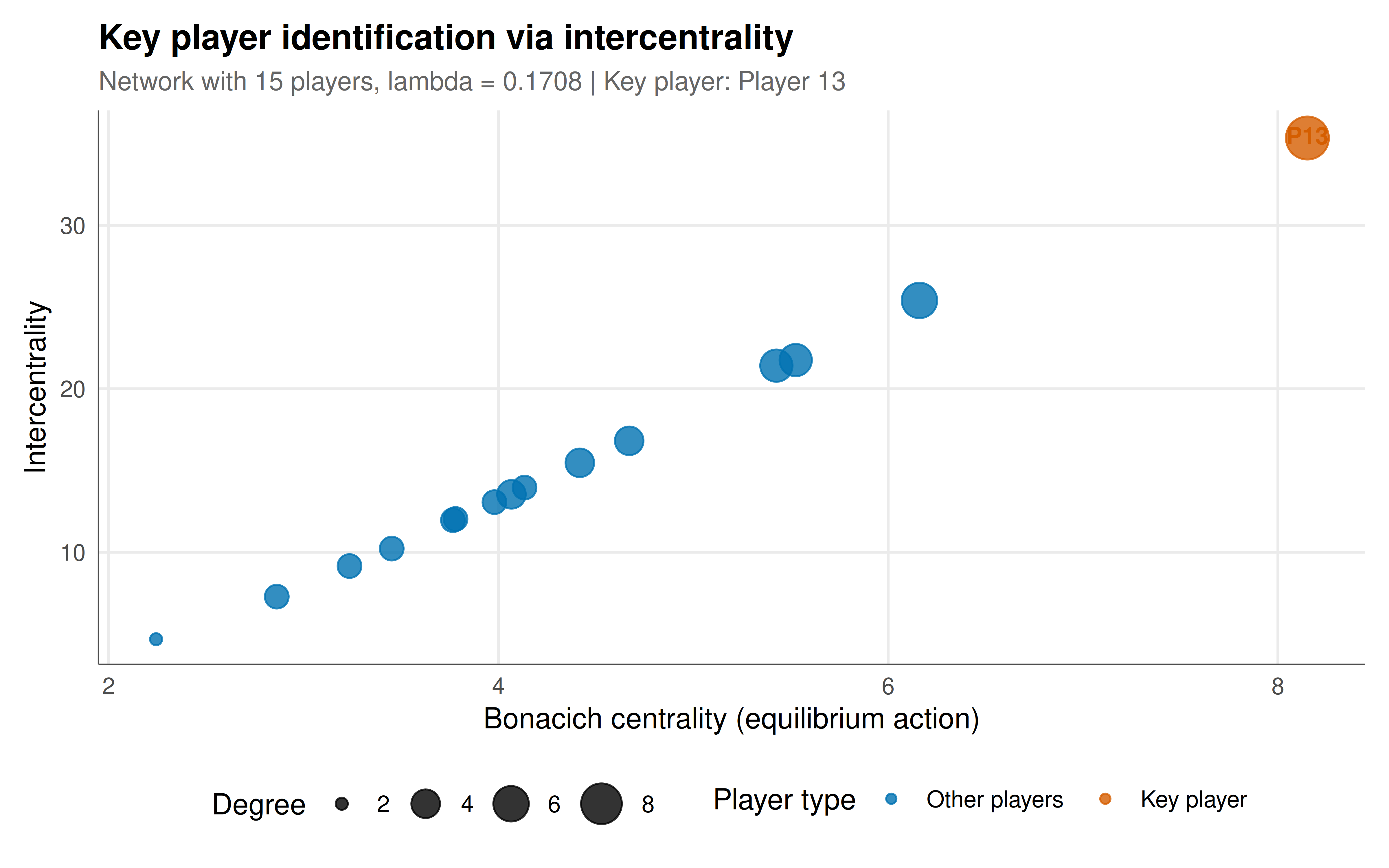
The figure displays the intercentrality versus Bonacich centrality for each player, with node size proportional to degree and the key player highlighted.
```{r}
#| label: fig-key-player-static
#| fig-cap: "Figure 1. Intercentrality versus Bonacich centrality for 15 players in a random network game with strategic complements. Point size reflects node degree. The key player (highlighted) maximises intercentrality, meaning their removal causes the largest drop in aggregate equilibrium activity. Note that the key player need not have the highest Bonacich centrality or degree. Okabe-Ito palette."
#| dev: [png, pdf]
#| fig-width: 8
#| fig-height: 5
#| dpi: 300
player_df$label <- ifelse(player_df$is_key,
                           paste0("Player ", player_df$player, " (Key)"),
                           paste0("Player ", player_df$player))

p <- ggplot(player_df, aes(x = bonacich, y = intercentrality,
                            size = degree, colour = is_key,
                            text = paste0("Player: ", player,
                                          "\nDegree: ", degree,
                                          "\nBonacich: ", bonacich,
                                          "\nIntercentrality: ", intercentrality))) +
  geom_point(alpha = 0.8) +
  geom_text(data = filter(player_df, is_key),
            aes(label = paste0("P", player)), nudge_y = 0.15,
            size = 3.5, colour = okabe_ito[6], fontface = "bold",
            show.legend = FALSE) +
  scale_colour_manual(values = c("FALSE" = okabe_ito[5], "TRUE" = okabe_ito[6]),
                      labels = c("Other players", "Key player"),
                      name = "Player type") +
  scale_size_continuous(range = c(2, 8), name = "Degree") +
  labs(title = "Key player identification via intercentrality",
       subtitle = paste0("Network with ", n, " players, lambda = ",
                         round(lambda, 4), " | Key player: Player ", key_player),
       x = "Bonacich centrality (equilibrium action)",
       y = "Intercentrality") +
  theme_publication()
p
```
## Interactive figure
Hover over each point to identify individual players and compare their degree, Bonacich centrality, and intercentrality. This interactive view helps explore why network position, not just connectivity, determines strategic importance.
```{r}
#| label: fig-key-player-interactive
ggplotly(p, tooltip = "text") |>
  config(displaylogo = FALSE,
         modeBarButtonsToRemove = c("select2d", "lasso2d"))
```
## Interpretation
The analysis reveals several fundamental insights about strategic influence in networks that challenge naive intuitions based on simple connectivity measures. The key player, identified by maximising intercentrality, is not necessarily the most connected node or the one with the highest equilibrium action. This disconnect arises because intercentrality captures a subtle interaction effect: it measures not just how active a player is, but how much that player's activity is amplified by the network structure and how much removing them would restructure the equilibrium for everyone else.
The Bonacich centrality vector provides the equilibrium actions directly, and it already accounts for network effects: a player connected to well-connected neighbours will have a higher Bonacich centrality than a player with the same degree but connected to peripheral nodes. This is the essence of strategic complements in networks -- high activity by neighbours encourages high activity by the focal player, and this effect propagates through paths of all lengths, with longer paths contributing proportionally to powers of the interaction parameter lambda. The closed-form expression through the Leontief inverse $(I - \lambda G)^{-1}$ elegantly captures this infinite series of direct and indirect effects.
Intercentrality goes one step further by accounting for what happens when a player is removed from the network. Removing a player does not simply subtract their activity from the total; it also eliminates all links incident to that player, which reduces the activity of their former neighbours, which in turn reduces the activity of their neighbours' neighbours, and so on through the network. The intercentrality measure, $b_i^2 / m_{ii}$, captures this cascading reduction. The numerator $b_i^2$ reflects the player's own equilibrium action (which is lost directly upon removal), while the denominator $m_{ii}$ adjusts for the network structure: a high diagonal element in the Leontief inverse indicates that the player's activity is substantially self-reinforced through network loops, and removing such a player has a disproportionately large cascading effect.
The policy implications are substantial. In criminal network interventions, targeting the key player rather than the most connected individual can achieve significantly larger reductions in total criminal activity. Our simulation shows that the key player's removal reduces aggregate activity by a meaningful percentage, whereas removing the highest-degree player would achieve a smaller reduction if the two differ. This difference can translate into substantial real-world impact: law enforcement resources are scarce, and directing them toward the strategically most important target maximises the return on intervention. Similar logic applies to vaccination campaigns in networks of social contact, where vaccinating the key player provides more herd immunity than vaccinating the most connected individual.
The parameter lambda plays a critical role in determining the network's strategic amplification. When lambda is small relative to the spectral radius, players' actions are only weakly coupled, and the key player is approximately the player with the highest degree. As lambda approaches the stability threshold $1/\rho(G)$, strategic complementarities become very strong, and the distinction between simple degree centrality and intercentrality becomes more pronounced. In this regime, the network topology matters enormously, and small differences in position can lead to large differences in strategic importance. This has implications for network design: organisations seeking to maximise aggregate effort should structure their internal networks to create strong positive feedback loops, while organisations seeking to minimise vulnerability to targeted disruption should favour decentralised, redundant network architectures.
## Extensions & related tutorials
The linear-quadratic framework extends to games with strategic substitutes (where lambda is negative), heterogeneous interaction strengths (weighted networks), and multiple equilibria in games with nonlinear best responses. Dynamic extensions model network formation as an endogenous process where players strategically choose their connections.
- [Eigenvalue methods for repeated game analysis](../../linear-algebra-matrix/eigenvalue-methods-repeated-games/)
- [World trade data for strategic analysis](../../public-apis-and-datasets/world-trade-strategic-data/)
- [Genetic algorithms for equilibrium computation](../../optimization-numerical-methods/genetic-algorithm-equilibria/)
- [Unit testing game theory solvers in R](../../r-package-development/unit-testing-game-solvers/)
## References
::: {#refs}
:::