---
title: "Monte Carlo methods for equilibrium computation"
description: "Use Monte Carlo simulation in R to approximate Nash equilibria, estimate equilibrium payoffs under uncertainty, and validate analytical solutions through large-sample simulation experiments."
author: "Raban Heller"
date: 2026-05-08
date-modified: 2026-05-08
categories:
- simulations
- monte-carlo
- equilibrium-computation
- numerical-methods
keywords: ["Monte Carlo", "simulation", "Nash equilibrium", "stochastic", "numerical methods", "convergence"]
labels: ["simulation-methods", "computational-gt"]
tier: 1
bibliography: ../../../references.bib
vgwort: "TODO_VGWORT_simulations_monte-carlo-game-equilibria"
image: thumbnail.png
image-alt: "Monte Carlo convergence of equilibrium payoff estimates with increasing sample size"
citation:
type: webpage
url: https://cttir.github.io/equilibria/tutorials/simulations/monte-carlo-game-equilibria/
license: "CC BY 4.0"
draft: false
has_static_fig: true
has_interactive_fig: true
has_shiny_app: false
---
```{r}
#| label: setup
#| include: false
library(ggplot2)
library(dplyr)
library(tidyr)
library(plotly)
okabe_ito <- c("#E69F00", "#56B4E9", "#009E73", "#F0E442",
"#0072B2", "#D55E00", "#CC79A7", "#999999")
theme_publication <- function(base_size = 12) {
theme_minimal(base_size = base_size) +
theme(plot.title = element_text(size = base_size * 1.2, face = "bold"),
plot.subtitle = element_text(size = base_size * 0.9, color = "grey40"),
axis.line = element_line(color = "grey30", linewidth = 0.3),
panel.grid.minor = element_blank(), legend.position = "bottom",
plot.margin = margin(10, 10, 10, 10))
}
```
## Introduction & motivation
Analytical solutions for game-theoretic equilibria exist only for special cases — symmetric games, small strategy spaces, or games with particular structural properties. For larger or more complex games — those with many players, continuous action spaces, stochastic payoffs, or incomplete information — exact computation may be intractable. **Monte Carlo simulation** provides a powerful alternative: rather than solving the game analytically, we simulate thousands or millions of plays and estimate equilibrium properties from the resulting sample. This approach is particularly valuable in three contexts. First, **validation**: we can verify analytical equilibrium predictions by simulating the game under equilibrium strategies and checking that payoffs, winning probabilities, and other statistics match the theory. Second, **approximation**: when the equilibrium is known in functional form but expected payoffs involve complex integrals (common in auction theory and Bayesian games), Monte Carlo integration provides numerical answers. Third, **exploration**: when the equilibrium is unknown, we can search over strategy spaces using simulation-based optimisation to find approximate equilibria. This tutorial simulates Matching Pennies at its known mixed equilibrium and a first-price auction with independent Beta(2,5) private values. It demonstrates payoff estimation, pointwise confidence intervals, and the relationship between sample size and precision. It does not search for an unknown equilibrium or implement variance reduction.
## Mathematical formulation
For a game with strategy profile $s = (s_1, \ldots, s_n)$ and payoff functions $u_i(s, \omega)$ where $\omega$ represents random elements (types, nature's moves), the **expected payoff** under strategy profile $s$ is:
$$E[u_i(s)] = \int u_i(s, \omega) \, dF(\omega)$$
The Monte Carlo estimator with $M$ samples is:
$$\hat{u}_i^M = \frac{1}{M} \sum_{m=1}^M u_i(s, \omega_m), \quad \omega_m \sim F$$
By the central limit theorem, $\hat{u}_i^M \xrightarrow{d} N(E[u_i], \sigma^2/M)$, giving a 95% confidence interval:
$$\hat{u}_i^M \pm 1.96 \cdot \frac{\hat{\sigma}}{\sqrt{M}}$$
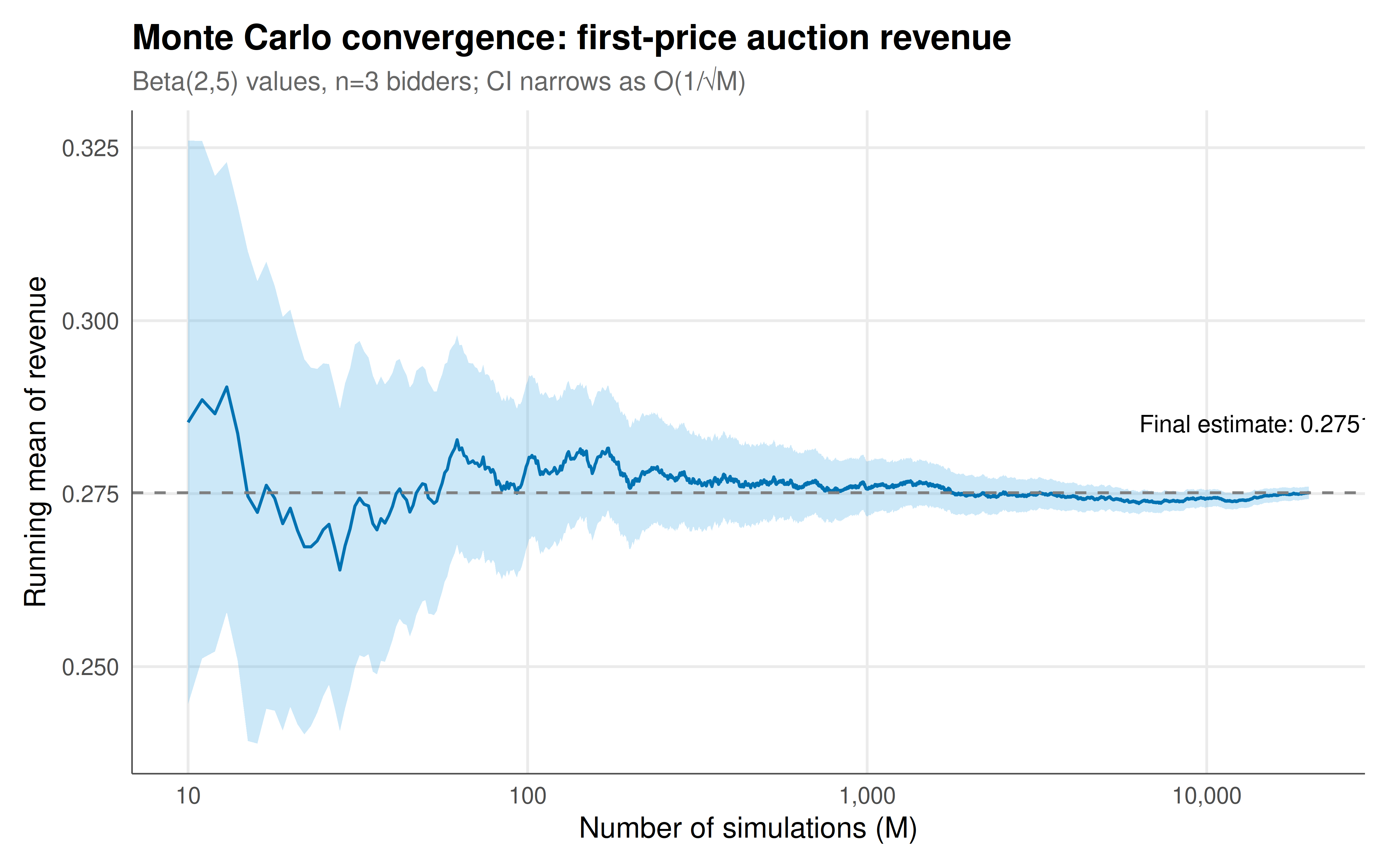
The **convergence rate** is $O(1/\sqrt{M})$: halving the confidence interval width requires quadrupling the sample size — a fundamental limitation of Monte Carlo methods.
For **equilibrium search**, we define a strategy $s_i$ parameterised by $\phi_i$ and search for $\phi^*$ such that no player can improve by deviating:
$$\phi_i^* = \arg\max_{\phi_i} \hat{u}_i^M(\phi_i, \phi_{-i}^*)$$
## R implementation
```{r}
#| label: monte-carlo-games
set.seed(42)

# === 1. Validation: Mixed-strategy NE in Matching Pennies ===
# NE: both mix 50-50. Expected payoff = 0 for both players.
n_sims <- c(100, 500, 1000, 5000, 10000, 50000)

mc_matching_pennies <- function(M) {
  p1 <- sample(c(1, -1), M, replace = TRUE)  # H=1, T=-1
  p2 <- sample(c(1, -1), M, replace = TRUE)
  payoff1 <- ifelse(p1 == p2, 1, -1)  # P1 wins if match
  c(mean = mean(payoff1), se = sd(payoff1) / sqrt(M))
}

cat("=== Monte Carlo Validation: Matching Pennies (NE: both mix 50-50) ===\n")
mp_results <- sapply(n_sims, mc_matching_pennies)
for (i in seq_along(n_sims)) {
  cat(sprintf("  M = %6d: mean = %+.4f, SE = %.4f, 95%% CI = [%.4f, %.4f]\n",
              n_sims[i], mp_results[1,i], mp_results[2,i],
              mp_results[1,i] - 1.96*mp_results[2,i],
              mp_results[1,i] + 1.96*mp_results[2,i]))
}
# === 2. Approximation: First-price auction with Beta-distributed values ===
# Values ~ Beta(2,5), n=3 bidders. Analytical BNE is complex; MC estimates revenue.
n_bidders <- 3
n_auction_sims <- 20000

# Symmetric independent-private-values equilibrium:
# b(v) = v - integral_0^v F(t)^(n-1) dt / F(v)^(n-1).
# Integrate once on a grid concentrated near zero, then interpolate bids.
# Quadrature/interpolation error is separate from Monte Carlo sampling error.
make_beta_bid <- function(n, a_shape = 2, b_shape = 5, n_grid = 20001L) {
  stopifnot(length(n) == 1L, is.finite(n), n >= 2, n == floor(n),
            length(a_shape) == 1L, is.finite(a_shape), a_shape > 0,
            length(b_shape) == 1L, is.finite(b_shape), b_shape > 0,
            length(n_grid) == 1L, is.finite(n_grid), n_grid >= 100,
            n_grid == floor(n_grid))
  grid <- seq(0, 1, length.out = n_grid)^2
  cdf_power <- pbeta(grid, a_shape, b_shape)^(n - 1)
  integral <- c(0, cumsum(diff(grid) *
                          (head(cdf_power, -1) + tail(cdf_power, -1)) / 2))
  bid <- numeric(length(grid))
  positive <- cdf_power > 0
  bid[positive] <- grid[positive] - integral[positive] / cdf_power[positive]
  bid <- pmax(0, pmin(grid, bid))
  interpolate <- approxfun(grid, bid, rule = 1)
  function(v) {
    if (!is.numeric(v) || any(!is.finite(v)) || any(v < 0 | v > 1))
      stop("Values must be finite numbers between zero and one.")
    interpolate(v)
  }
}
bid_fpa_beta <- make_beta_bid(n_bidders)
values <- matrix(rbeta(n_bidders * n_auction_sims, 2, 5), nrow = n_auction_sims)
bids <- matrix(bid_fpa_beta(as.vector(values)), nrow = n_auction_sims)

winners <- apply(bids, 1, which.max)
revenues <- bids[cbind(1:n_auction_sims, winners)]
winner_values <- values[cbind(1:n_auction_sims, winners)]
surpluses <- winner_values - revenues

cat(sprintf("\n=== First-Price Auction: Beta(2,5) values, n=%d bidders, M=%d ===\n",
            n_bidders, n_auction_sims))
cat(sprintf(" Mean revenue: %.4f (SE: %.4f)\n", mean(revenues), sd(revenues)/sqrt(n_auction_sims)))
cat(sprintf(" Mean winner surplus: %.4f\n", mean(surpluses)))
cat(sprintf(" Mean winner value: %.4f\n", mean(winner_values)))
cat(sprintf("  Efficiency (winner has highest value): %.1f%%\n",
            100 * mean(apply(values, 1, which.max) == winners)))
# === 3. Convergence tracking ===
# Track running mean of auction revenue as M grows
running_means <- cumsum(revenues) / (1:n_auction_sims)
sample_count <- seq_along(revenues)
running_variance <- pmax(0, cumsum(revenues^2) - sample_count * running_means^2) /
  pmax(1, sample_count - 1)
running_se <- sqrt(running_variance / sample_count)
running_se[1] <- NA_real_


cat(sprintf("\n  Convergence: at M=100: %.4f, M=1000: %.4f, M=10000: %.4f, M=20000: %.4f\n",
            running_means[100], running_means[1000], running_means[10000], running_means[20000]))
```
## Static publication-ready figure
```{r}
#| label: fig-mc-convergence
#| fig-cap: "Figure 1. Monte Carlo convergence of expected revenue in a first-price auction with Beta(2,5) values and 3 bidders. The running mean (blue) estimates revenue under the numerically approximated bidding strategy. The shaded intervals are pointwise normal approximations; they are not a simultaneous confidence band and exclude numerical integration error. The inset text shows the final estimate. This demonstrates the fundamental trade-off in Monte Carlo methods: more precision requires quadratically more computation. Okabe-Ito palette."
#| dev: [png, pdf]
#| fig-width: 8
#| fig-height: 5
#| dpi: 300
conv_df <- tibble(
  M = 1:n_auction_sims,
  running_mean = running_means,
  se = running_se,
  lower = running_mean - 1.96 * se,
  upper = running_mean + 1.96 * se
) |> filter(M >= 10)  # skip first few for stability

final_est <- tail(running_means, 1)

ggplot(conv_df, aes(x = M)) +
  geom_ribbon(aes(ymin = lower, ymax = upper), fill = okabe_ito[2], alpha = 0.3) +
  geom_line(aes(y = running_mean), color = okabe_ito[5], linewidth = 0.6) +
  geom_hline(yintercept = final_est, linetype = "dashed", color = "grey50") +
  annotate("text", x = n_auction_sims * 0.7, y = final_est + 0.01,
           label = sprintf("Final estimate: %.4f", final_est), size = 3.5) +
  scale_x_log10(labels = scales::comma_format()) +
  labs(title = "Monte Carlo convergence: first-price auction revenue",
       subtitle = sprintf("Beta(2,5) values, n=3 bidders; CI narrows as O(1/√M)"),
       x = "Number of simulations (M)", y = "Running mean of revenue") +
  theme_publication()
```
## Interactive figure
```{r}
#| label: fig-mc-sample-size
# Compare MC precision across different sample sizes for multiple game statistics
sample_sizes <- c(50, 100, 200, 500, 1000, 2000, 5000, 10000)
n_reps <- 200  # replications per sample size

precision_data <- lapply(sample_sizes, function(M) {
  reps <- replicate(n_reps, {
    vals <- matrix(rbeta(n_bidders * M, 2, 5), nrow = M)
    # Monotone symmetric bids make the highest-value bidder the winner.
    winner_value <- do.call(pmax, as.data.frame(vals))
    rev <- bid_fpa_beta(winner_value)
    mean(rev)
  })
  tibble(M = M, mean_est = mean(reps), sd_est = sd(reps),
         cv = sd(reps) / mean(reps) * 100)
}) |> bind_rows() |>
  mutate(text = paste0("M = ", M,
                       "\nMean revenue: ", round(mean_est, 4),
                       "\nSD of estimates: ", round(sd_est, 4),
                       "\nCV: ", round(cv, 2), "%"))

p_precision <- ggplot(precision_data, aes(x = M, y = sd_est, text = text)) +
  geom_line(color = okabe_ito[5], linewidth = 1) +
  geom_point(color = okabe_ito[5], size = 3) +
  scale_x_log10() +
  scale_y_log10() +
  labs(title = "Monte Carlo precision vs sample size",
       subtitle = "SD of revenue estimates across 200 replications; log-log scale shows 1/√M slope",
       x = "Sample size (M)", y = "Standard deviation of estimates") +
  theme_publication()

ggplotly(p_precision, tooltip = "text") |>
  config(displaylogo = FALSE, modeBarButtonsToRemove = c("select2d", "lasso2d"))
```
## Interpretation
The Matching Pennies example estimates the zero payoff implied by independently mixing 50–50. The auction uses the symmetric risk-neutral equilibrium formula for independent private values, approximated by trapezoidal integration on a fixed grid. The bids are computed once and interpolated for every simulated value, avoiding millions of repeated numerical integrations. Regression checks compare the bids with adaptive numerical integrals and the closed-form uniform-value auction.
There are two distinct error sources: numerical approximation of the bidding function and Monte Carlo estimation of revenue. The plotted standard errors describe sampling uncertainty only. At a fixed sample size, the normal intervals are asymptotic pointwise intervals; inspecting many successive intervals does not give simultaneous 95% coverage. These draws are independent, so a stationary-regime or burn-in diagnostic is not relevant.
The repeated-sampling plot estimates how the standard deviation changes with sample size. The expected rate is $O(M^{-1/2})$ when variance is finite. A precision target should use the estimated standard error relative to the estimated revenue, rather than a universal sample-size prescription. Antithetic sampling, control variates, and importance sampling are possible extensions; this tutorial does not measure their benefit or establish an unknown equilibrium.
## Extensions & related tutorials
- [Spatial Prisoner's Dilemma — Nowak & May](../spatial-prisoners-dilemma-nowak-may/) — agent-based simulation of evolutionary dynamics.
- [First-price auction equilibrium](../../auction-theory-deep-dive/first-price-sealed-bid/) — analytical equilibrium validated by MC.
- [Revenue equivalence theorem](../../auction-theory-deep-dive/revenue-equivalence/) — MC verification across auction formats.
- [Moran process in finite populations](../../evolutionary-gt/moran-process-finite-populations/) — stochastic simulation of evolutionary dynamics.
- [Bootstrap methods for game theory](../../statistical-foundations/bootstrap-game-theory/) — resampling-based inference.
## References
::: {#refs}
:::