Spectral Density

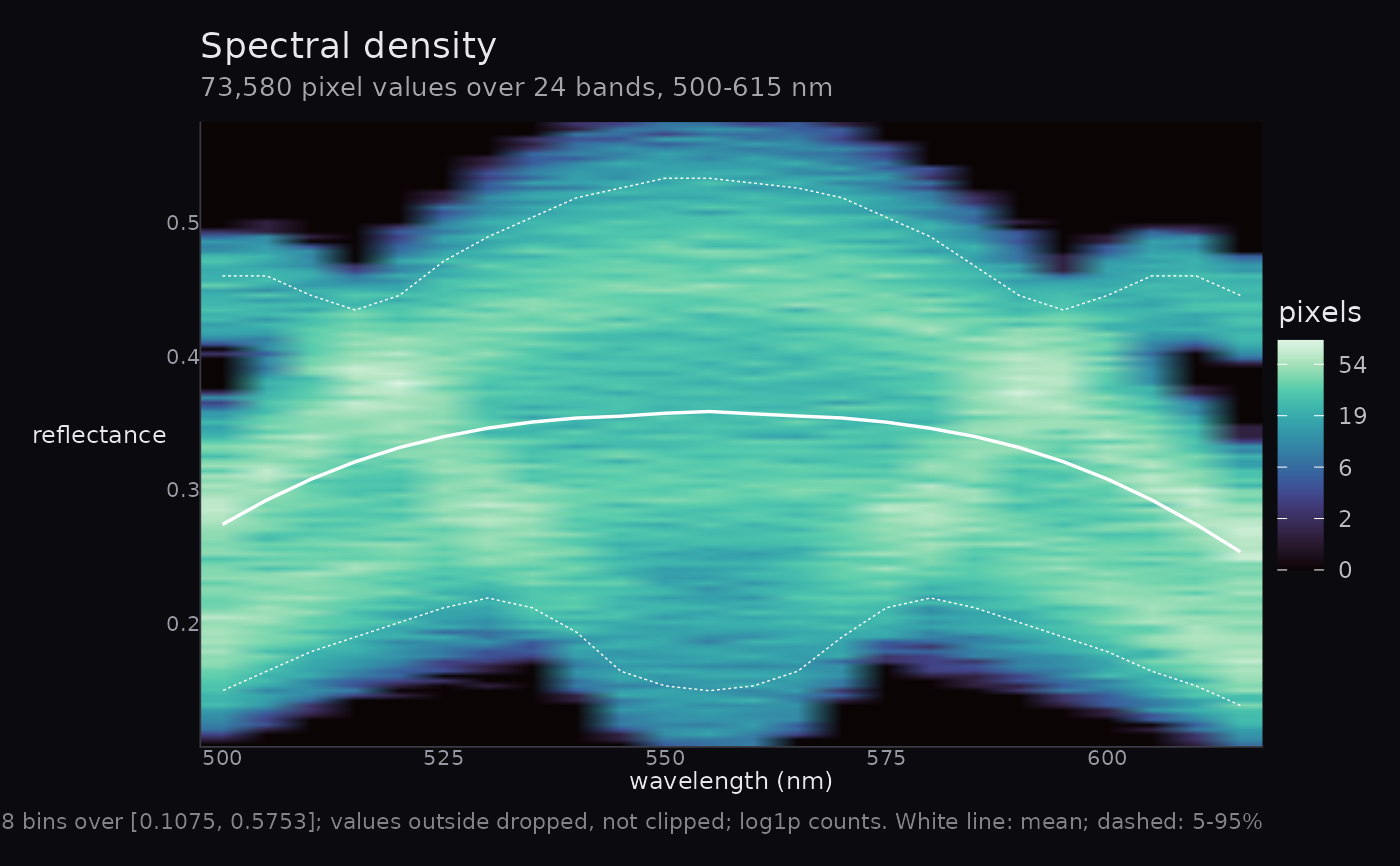
Draws the joint distribution of input values and spectral coordinates as an exact two-dimensional histogram. A binned mean and binned 5–95% pixel envelope are calculated from the retained histogram counts.

Usage

hsa_spectral_density(
  cube,
  nbins = 128L,
  limits = NULL,
  transform = c("log1p", "identity"),
  normalise = c("none", "band"),
  palette = "mako",
  show_limits = FALSE,
  probs = c(0.02, 0.98),
  value_label = "input value"
)

Arguments

cube

An hsi_cube (from hyperspectR) or a 3-D array with dimensions (rows, cols, bands), of integer or double values. Optional wavelengths metadata must be finite, unique and strictly increasing in nm. Without it, coordinates are band indices. An optional logical spatial mask has dimensions (rows, cols) and no missing entries; FALSE excludes a pixel. Arrays may carry these as attributes; an hsi_cube may carry them as list fields. Nonfinite observations are excluded.

nbins

Number of value bins. Must be an integer of at least two. Default 128.

limits

Numeric length-two value range to bin over. NULL (default) uses the 0.1st and 99.9th percentiles of all finite eligible values.

transform

Display transform: "log1p" (default) or "identity". Legend labels are returned to raw counts or shares.

normalise

"none" (default) displays raw counts; "band" displays shares of the retained count in each band. Empty bands remain missing.

palette

Palette name passed to hsa_palette().

show_limits

Logical. Draw global raw eligible-value percentiles using probs. These references include finite observations outside limits and are separate from image enhancement limits. Default FALSE.

probs

Two increasing finite probabilities between zero and one for the global raw eligible-value references when show_limits = TRUE. These do not set the histogram range or image enhancement limits.

value_label

A truthful label for the input values. Default "input value". A reflectance label requires known upstream calibration; numeric range alone cannot establish calibration.

Value

A ggplot2 object with compact original-rendering provenance.

Details

Values outside limits are dropped rather than clipped into the end bins. Masks and nonfinite values are excluded. The overlay describes the retained pixel distribution; it is not a confidence interval.

Examples

cube <- hsa_demo_cube()
hsa_spectral_density(cube)