


Two independent groups of fixed size, each with a binary outcome, give a two-by-two table. Fisher’s exact test conditions on both margins of that table. Boschloo’s unconditional test (Boschloo, 1970) uses Fisher’s p-value only to order the possible tables. Its p-value is the largest probability, over all values of the common event probability under the null hypothesis, of a table at least as extreme as the observed one. With the same sidedness convention, Boschloo’s p-value never exceeds Fisher’s.
This tutorial computes Boschloo’s test with infercalcR, compares it with Fisher’s test and looks at the rejection region of a design. The calculations use only base R. One section uses the optional package digest and is evaluated only when it is installed.
has_digest <- requireNamespace("digest", quietly = TRUE)The observed table
In this synthetic example, 2 of 12 patients respond in the control group and 8 of 12 in the treatment group. Rows are groups; the first column counts the events.
Choose a variant before looking at the data
The two-sided alternative can be defined in two ways, and there are
two one-sided alternatives. boschloo_variants() lists the
variants and how each orders the tables.
variants <- boschloo_variants()
variants[, c("variant", "alternative", "label")]
#>   variant alternative
#> 1 minlike    p1 != p2
#> 2 central    p1 != p2
#> 3    less     p1 < p2
#> 4 greater     p1 > p2
#>                                                                     label
#> 1   Boschloo test, two-sided, minlike ordering (two-sided Fisher p-value)
#> 2 Boschloo test, two-sided, central (twice the smaller one-sided p-value)
#> 3                                   Boschloo test, one-sided, H1: p1 < p2
#> 4                                   Boschloo test, one-sided, H1: p1 > p2
The minlike variant orders tables by the two-sided
Fisher p-value. The central variant doubles the smaller of
the two one-sided p-values. Group 1 is the first group passed to the
function, so less means that the event probability in group
1 is lower than in group 2.
Compute the test
boschloo_inference() takes the event counts and group
sizes and returns a result in the common contract described in the getting-started tutorial.
boschloo <- boschloo_inference(x1 = 2, n1 = 12, x2 = 8, n2 = 12,
                               variant = "minlike", alpha = 0.05,
                               groups = c("control", "treatment"),
                               event = "response")
print(result_data(boschloo)[, c("estimand", "contrast", "estimate", "p.value",
                                "p.upper", "decision", "status")],
      row.names = FALSE)
#>                                              estimand            contrast
#>  event probability difference (group 1 minus group 2) control - treatment
#>  estimate    p.value    p.upper decision status
#>      -0.5 0.01688614 0.01688614   reject     ok
The estimate is the observed difference in event proportions, control
minus treatment. The p-value is a supremum over the nuisance parameter
and is found numerically. p.value is the largest value
attained by the search and p.upper is a guaranteed upper
bound for the supremum. The decision at the stated alpha
uses the upper bound. The bound describes numerical precision only; it
is not a confidence interval. The metadata state the assumptions.
meta <- result_metadata(boschloo)
meta$assumptions
#> [1] "two independent binomial samples with fixed group sizes; not for paired or matched binary data (McNemar-type tests)"
meta$numerical_bounds
#> [1] "p.value is attained lower bound; p.upper is rigorous numerical upper bound, not a sampling interval"
boschloo$payload$native$fisher_p_value
#> [1] 0.03607484
The last value is Fisher’s two-sided p-value for the same table, kept for comparison. Boschloo’s p-value is smaller here.
The same test through a method specification
The Boschloo variants are also available through
method_spec() and run_inference(), which take
the table directly.
minlike_spec <- method_spec("boschloo_two_sided_minlike")
via_spec <- run_inference(minlike_spec, table = responses)
print(result_data(via_spec)[, c("estimand", "estimate", "p.value")],
      row.names = FALSE)
#>                                                               estimand estimate
#>  Boschloo test, two-sided, minlike ordering (two-sided Fisher p-value)       NA
#>              observed event probability difference (row 1 minus row 2)     -0.5
#>     p.value
#>  0.01688614
#>          NA
stopifnot(isTRUE(all.equal(result_data(via_spec)$p.value[1],
                           result_data(boschloo)$p.value)))
This result has one row for the test and one for the observed
difference in proportions. One-sided tests use
boschloo_one_sided with the alternative declared in the
specification.
less_spec <- method_spec("boschloo_one_sided", alternative = "less")
less <- run_inference(less_spec, table = responses)
result_data(less)[1, c("estimand", "p.value", "alternative")]
#>                                estimand     p.value alternative
#> 1 Boschloo test, one-sided, H1: p1 < p2 0.008443069        less
Sidedness matters
The variants answer different questions. For this table the two two-sided variants happen to agree, while the one-sided p-values depend strongly on the direction. Choose the variant in the analysis plan.
p_values <- vapply(c("minlike", "central", "less", "greater"), function(v) {
  result_data(boschloo_inference(2, 12, 8, 12, variant = v))$p.value
}, numeric(1))
round(p_values, 5)
#> minlike central    less greater
#> 0.01689 0.01689 0.00844 0.99526
Compare with other exact tests
Fisher’s exact test is available through the same interface and
agrees with stats::fisher.test().
fisher <- run_inference(method_spec("fisher_exact_2x2"), table = responses)
print(result_data(fisher)[, c("estimand", "estimate", "conf.low", "conf.high",
                              "p.value")],
      row.names = FALSE)
#>                                      estimand  estimate    conf.low conf.high
#>  conditional event odds ratio (row 1 / row 2) 0.1121872 0.008101526  0.896925
#>     p.value
#>  0.03607484
stopifnot(isTRUE(all.equal(result_data(fisher)$p.value,
                           stats::fisher.test(responses)$p.value)))
Another unconditional exact test orders the tables by the pooled Z statistic instead of Fisher’s p-value. It requires an explicit statement that the two groups are independent binomial samples.
z_pooled <- run_inference(method_spec("unconditional_exact_z_pooled"),
                          table = responses,
                          independent_binomial_groups = TRUE)
print(result_data(z_pooled)[, c("estimand", "estimate", "p.value")],
      row.names = FALSE)
#>                                                   estimand estimate    p.value
#>                          Unconditional exact pooled-Z test       NA 0.01743367
#>  observed event probability difference (row 1 minus row 2)     -0.5         NA
Operating characteristics of a design
For a planned design with 12 units per group,
boschloo_compare_fisher() compares the rejection regions of
the two tests at the same nominal level. The attained size is the
largest probability of rejecting the null hypothesis over all common
event probabilities. Power is computed at event probabilities that the
analyst supplies.
comparison <- boschloo_compare_fisher(n1 = 12, n2 = 12, alpha = 0.05,
                                      variant = "minlike", p1 = 0.2, p2 = 0.6)
comparison
#> <boschloo_fisher_comparison> Boschloo test, two-sided, minlike ordering (two-sided Fisher p-value) vs Fisher (same sidedness convention as the Boschloo variant)
#>   design n1 = 12, n2 = 12, alpha = 0.05
#>   rejected by both: 60; Boschloo only: 12; Fisher only: 0; neither: 97
#>   attained size: Boschloo 0.0449066, Fisher 0.0228447
#>   power at p1 = 0.2, p2 = 0.6: Boschloo 0.498862, Fisher 0.391534
For this design, every table rejected by Fisher’s test is also rejected by Boschloo’s test. The additional tables bring the attained size closer to the nominal 5 % and increase the power.
boschloo_plotdata_lattice() returns one row per possible
table of the design, with its Boschloo p-value and whether it is in the
rejection region. The observed table can be marked.
lattice <- boschloo_plotdata_lattice(12, 12, alpha = 0.05, variant = "minlike",
                                     observed = c(x1 = 2, x2 = 8))
tables <- lattice$data
lattice$reference[c("attained_size", "n_rejected")]
#> $attained_size
#> [1] 0.04490661
#>
#> $n_rejected
#> [1] 72
plot(tables$x1, tables$x2, pch = ifelse(tables$in_region, 15, 0),
     xlab = "Events in group 1 (control)", ylab = "Events in group 2 (treatment)",
     main = "Rejection region, n = 12 per group", asp = 1)
points(tables$x1[tables$observed], tables$x2[tables$observed], cex = 2.5, lwd = 2)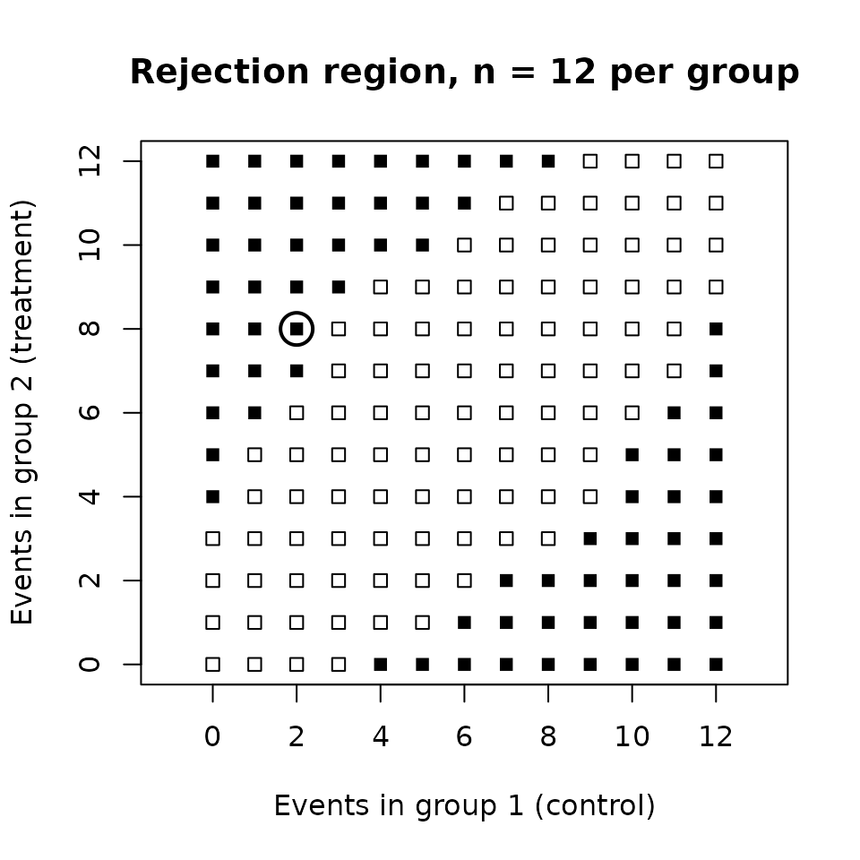
A complete test record
boschloo_test() returns the full record of the
calculation, including the numerical settings and a fingerprint of the
specification. The fingerprint uses digest.
record <- boschloo_test(2, 12, 8, 12, variant = "minlike", alpha = 0.05,
                        groups = c("control", "treatment"), event = "response")
record
#> <boschloo_test> Boschloo test, two-sided, minlike ordering (two-sided Fisher p-value)
#>   data:        group 1 = control (x1 = 2 of n1 = 12), group 2 = treatment (x2 = 8 of n2 = 12); events = response
#>   H0: p1 = p2;  H1: p1 != p2
#>   status:      ok
#>   p-value:     0.01688614 (rigorous upper bound 0.01688614)
#>   decision at alpha = 0.05: reject
#>   Fisher p (same convention, comparison only): 0.03607484
#>   minlike tail: sup at pi = 0.50803; ordering statistic 0.03607484; tail of 54 tables; floating_tolerance ordering
#>   settings:    tie tolerance 1e-07; 1001 grid points + bisection; bound tolerance 1e-09
#>   scope:       observed data: p-value of the observed table; no planning quantity
The p-value is the maximum of the null probability of the tail set
over the common event probability.
boschloo_plotdata_nuisance() evaluates that curve.
nuisance <- boschloo_plotdata_nuisance(record, grid_points = 201)
plot(nuisance$data$pi, nuisance$data$probability, type = "l",
     xlab = "Common event probability", ylab = "Null probability of tail set")
abline(h = record$p_value, lty = 2)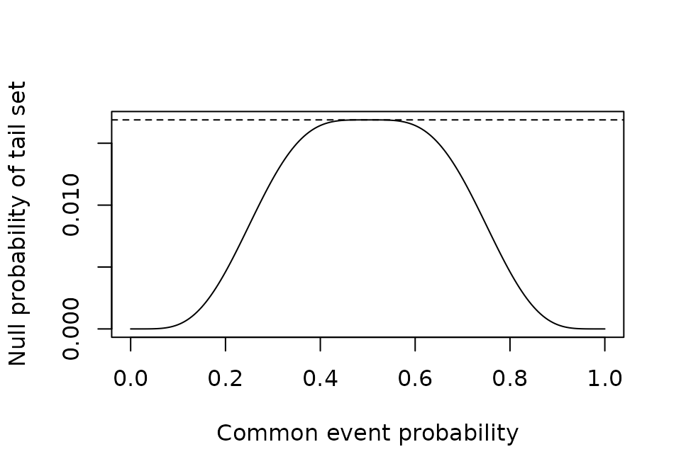
The record converts to the common contract with
as_inference().
common <- as_inference(record)
stopifnot(isTRUE(all.equal(result_data(common)$p.value,
                           result_data(boschloo)$p.value)))
The numerical tolerances of the search are set with
boschloo_control() and stored with every result.
boschloo_control()
#> <boschloo_control>
#>   tie tolerance (relative): 1e-07
#>   nuisance grid points:     1001 (plus branch-and-bound bisection)
#>   supremum bound tolerance: 1e-09
#>   Brent polish tolerance:   1e-12
#>   ambiguity band:           (1e-12, 1e-06]
#>   cache:                    TRUE
Reference
Boschloo, R. D. (1970). Raised conditional level of significance for the 2 x 2-table when testing the equality of two probabilities. Statistica Neerlandica, 24(1), 1-9. https://doi.org/10.1111/j.1467-9574.1970.tb00104.x
Acknowledgments and sources
This package is part of an inference suite (infercalcR, inferguidR and infereportR) that is deeply inspired by DescrTab2 [1], developed at the Institute of Medical Biometry (IMBI), Heidelberg University, by Jan Meis, Lukas Baumann, Maximilian Pilz and Lukas Sauer. Its test-choice tree, its validation statement and its practice of computing each test with an established implementation are the model for how the suite chooses, computes and reports statistical tests. DescrTab2 was archived on CRAN on 18 October 2025; its source code remains available on GitHub. The methods-consulting pages of the University of Zurich [2], with their decision tree, decision assistant, worked examples and explanations, inspired the guidance in the suite. Power and sample-size planning and the distribution calculator follow G*Power 3.1 [3, 4]. We thank the authors of these works for making them openly available. The package README cites all software the package uses.
- Meis J, Baumann L, Pilz M, Sauer L (2022). DescrTab2: Publication Quality Descriptive Statistics Tables. R package version 2.1.16. https://doi.org/10.32614/CRAN.package.DescrTab2. Source code, including the development version 2.1.26: https://github.com/imbi-heidelberg/DescrTab2.
- Universität Zürich, Methodenberatung. Datenanalyse mit SPSS: decision tree (Entscheidbaum), decision assistant (Entscheidassistent) and method pages with examples and explanations. https://www.methodenberatung.uzh.ch/de/datenanalyse_spss.html. Accessed 3 October 2026.
- Faul F, Erdfelder E, Lang A-G, Buchner A (2007). G*Power 3: A flexible statistical power analysis program for the social, behavioral, and biomedical sciences. Behavior Research Methods, 39(2), 175-191. https://doi.org/10.3758/BF03193146.
- Faul F, Erdfelder E, Buchner A, Lang A-G (2009). Statistical power analyses using G*Power 3.1: Tests for correlation and regression analyses. Behavior Research Methods, 41(4), 1149-1160. https://doi.org/10.3758/BRM.41.4.1149.
sessionInfo()
#> R version 4.6.2 (2026-10-29)
#> Platform: x86_64-pc-linux-gnu
#> Running under: Ubuntu 26.04.1 LTS
#>
#> Matrix products: default
#> BLAS:   /usr/lib/x86_64-linux-gnu/openblas-pthread/libblas.so.3
#> LAPACK: /usr/lib/x86_64-linux-gnu/openblas-pthread/libopenblasp-r0.3.32.so;  LAPACK version 3.12.0
#>
#> locale:
#>  [1] LC_CTYPE=C.UTF-8       LC_NUMERIC=C           LC_TIME=C.UTF-8
#>  [4] LC_COLLATE=C.UTF-8     LC_MONETARY=C.UTF-8    LC_MESSAGES=C.UTF-8
#>  [7] LC_PAPER=C.UTF-8       LC_NAME=C              LC_ADDRESS=C
#> [10] LC_TELEPHONE=C         LC_MEASUREMENT=C.UTF-8 LC_IDENTIFICATION=C
#>
#> time zone: UTC
#> tzcode source: system (glibc)
#>
#> attached base packages:
#> [1] stats     graphics  grDevices utils     datasets  methods   base
#>
#> other attached packages:
#> [1] infercalcR_0.1.0
#>
#> loaded via a namespace (and not attached):
#>  [1] digest_0.6.39     desc_1.4.3        R6_2.6.1          fastmap_1.2.0
#>  [5] xfun_0.62         cachem_1.1.0      knitr_1.52        htmltools_0.5.9
#>  [9] rmarkdown_2.32    lifecycle_1.0.5   cli_3.6.6         sass_0.4.10
#> [13] pkgdown_2.2.1     textshaping_1.0.5 jquerylib_0.1.4   systemfonts_1.3.2
#> [17] compiler_4.6.2    tools_4.6.2       ragg_1.5.2        bslib_0.12.0
#> [21] evaluate_1.0.5    yaml_2.3.12       otel_0.3.0        jsonlite_2.0.0
#> [25] rlang_1.3.0       fs_2.1.0