Getting Started with pressR • pressR

library(pressR)

What pressR does

pressR parses, analyzes, and visualizes pressure distribution data from capacitive sensor systems. It provides:

Predefined sensor layouts (in-shoe insoles, pressure platforms, saddle mats, seating mats, glove sensors),
Parsers for ASCII and CSV pressure data files,
A full analysis pipeline (per-frame metrics, trial summaries, regional analysis, gait-cycle detection, saddle-fit checks),
ggplot2-based visualization and composite reports,
An interactive Shiny application for data exploration.

Load a layout

Every trial is tied to a pr_layout object that describes the sensor geometry. For example, a 99-sensor in-shoe pressure insole:

layout <- pr_layout_insole()
print(layout)
#> 
#> ── pr_layout: insole_standard ──────────────────────────────────────────────────
#> In-shoe pressure insole (99 sensors, standard).
#> • Manufacturer: ""
#> • Model: "insole"
#> • Grid: 18 x 8
#> • Active sensors: 99
#> • Sensor area: 1.5 cm²
#> • Pressure range: 0 - 1200 kPa
#> • Regions: 7
#> Region names: "heel", "midfoot", "metatarsal_1", "metatarsal_2_3",
#> "metatarsal_4_5", "hallux", and "lesser_toes"

Generate a synthetic example trial

pr_example_trial() produces realistic synthetic data for each supported application. This is useful for quick demos, tests, and vignettes.

trial <- pr_example_trial("insole")
trial
#> 
#> ── pr_trial ────────────────────────────────────────────────────────────────────
#> • System: "insole"
#> • Layout: "insole_standard"
#> • Frames: 250
#> • Duration: 5 s
#> • Sampling: 50 Hz
#> • Sensors: 99
#> • Subject: "EX01"
#> • Date: "2026-05-04"
#> • Condition: "walking"

Visualize

The default plot method draws a maximum-pressure picture (MPP):

pr_plot_heatmap(trial)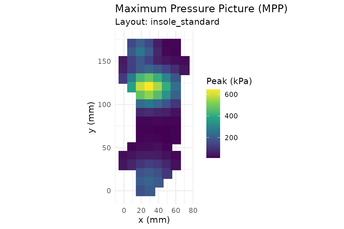

MPP heatmap of the synthetic insole trial

Time-domain curves are equally straightforward:

pr_plot_force_time(trial, show_cycles = TRUE)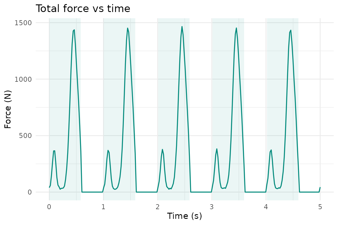

Force vs time with gait cycles shaded

Summarize

pr_summary() returns a single-row tibble containing the common biomechanical parameters:

pr_summary(trial)
#> # A tibble: 1 × 14
#>     mpp   mvp max_force mean_force max_contact_area mean_contact_area
#>   <dbl> <dbl>     <dbl>      <dbl>            <dbl>             <dbl>
#> 1  646.  43.0     1466.       289.             128.              60.9
#> # ℹ 8 more variables: contact_time <dbl>, pti_max <dbl>, pti_mean <dbl>,
#> #   impulse <dbl>, cop_path_length <dbl>, cop_velocity_mean <dbl>,
#> #   cop_range_ap <dbl>, cop_range_ml <dbl>

Regional analysis

With the insole layout’s default region masks you get one row per anatomical region:

pr_calc_regional(trial)
#> # A tibble: 7 × 6
#>   region           mpp   mvp max_force contact_area pti_mean
#>   <chr>          <dbl> <dbl>     <dbl>        <dbl>    <dbl>
#> 1 heel            220.  15.0     357.          42       40.2
#> 2 midfoot         646.  59.6    1248.          61.5    155. 
#> 3 metatarsal_1    130.  23.0      41.9          6       65.4
#> 4 metatarsal_2_3  224.  43.3     116.           9      127. 
#> 5 metatarsal_4_5  137.  15.9      49.1          9       43.8
#> 6 hallux          265.  29.9     120.           6       83.8
#> 7 lesser_toes     190.  12.9      73.1         12       30.0

Export

Results can be exported as CSV:

tmp <- tempfile(fileext = ".csv")
pr_export_csv(trial, tmp, what = "summary")

Launch the Shiny app

pr_run_app(trial)