Research-management analytics: coverage, attribution, and policy evaluation • scimapR

This article walks an end-to-end research-management study: auditing an institution’s publication output against a ground-truth tracker, capturing affiliations robustly, evaluating whether an intervention changed output, and summarising impact defensibly. Everything runs on synthetic example data.

A reproducible starting corpus

For arbitrary tabular sources, sm_corpus_from_tables() is the recommended ingestion path: it validates required columns, coerces types, fills missing optional tables, and returns a valid sm_corpus.

works <- data.frame(
  work_id = paste0("W", 1:4),
  title = c("Spatial transcriptomics in cancer",
            "Immune checkpoint resistance",
            "A trial of biomarker discovery",
            "Single-cell atlas of the tumour"),
  year = c("2018", "2019", "2020", "2021"),   # character -> coerced to integer
  doi = paste0("10.1234/example.", 1:4),
  cited_by_count = c(40, 12, 5, 1)
)
corpus <- sm_corpus_from_tables(list(works = works))
corpus

For the rest of the article we use the larger built-in synthetic corpus.

corpus <- sm_example_corpus(n_works = 200, seed = 1)

1. Coverage auditing

Suppose a manual tracker lists the works the institution should have. We can measure recall and precision of the corpus against it, and see which years are worst covered.

reference <- corpus$works[1:150, c("work_id", "doi", "title", "year")]
names(reference)[1] <- "id"

cov <- sm_coverage_audit(corpus, reference, by = "year", match = "doi")
cov
summary(cov)
#> # A tibble: 1 × 8
#>   recall precision    f1 n_corpus n_reference n_matched n_corpus_only
#>    <dbl>     <dbl> <dbl>    <int>       <int>     <int>         <int>
#> 1      1      0.75 0.857      200         150       150            50
#> # ℹ 1 more variable: n_reference_only <int>

ggplot2::autoplot(cov)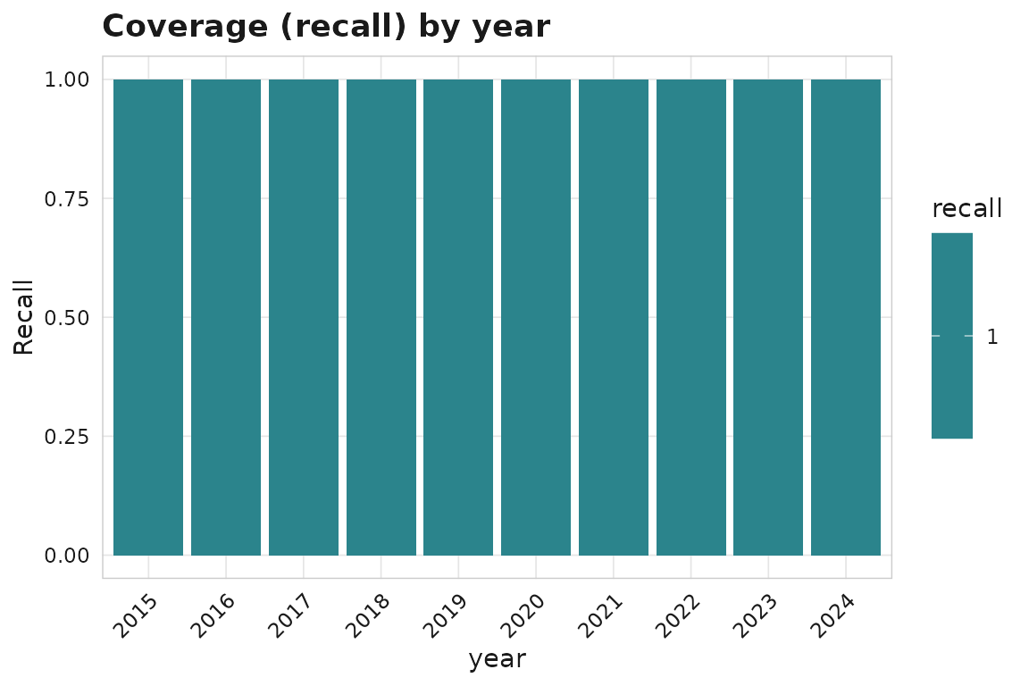

Breakdowns are returned as a single flat tibble; use sm_coverage_breakdowns() to access or filter them:

sm_coverage_breakdowns(cov, dimension = "year")
#> # A tibble: 10 × 8
#>    dimension level n_reference n_matched recall n_corpus precision    f1
#>    <chr>     <chr>       <int>     <int>  <dbl>    <int>     <dbl> <dbl>
#>  1 year      2015           18        18      1       24     0.75  0.857
#>  2 year      2016           12        12      1       17     0.706 0.828
#>  3 year      2017           15        15      1       20     0.75  0.857
#>  4 year      2018           16        16      1       20     0.8   0.889
#>  5 year      2019           19        19      1       25     0.76  0.864
#>  6 year      2020            9         9      1       15     0.6   0.75 
#>  7 year      2021           16        16      1       20     0.8   0.889
#>  8 year      2022           13        13      1       19     0.684 0.812
#>  9 year      2023           17        17      1       20     0.85  0.919
#> 10 year      2024           15        15      1       20     0.75  0.857

Source coverage can be checked against a journal master list by ISSN (sm_journal_in_index()), and two corpora reconciled by content with sm_reconcile().

ref_index <- utils::read.csv(
  system.file("extdata", "example_journal_index.csv", package = "scimapR"),
  stringsAsFactors = FALSE
)
sm_journal_in_index(c("1078-8956", "9999-9999"), index = "doaj",
                    reference_list = ref_index)
#> # A tibble: 2 × 5
#>   issn      index in_index matched_title   matched_issn_type
#>   <chr>     <chr> <lgl>    <chr>           <chr>            
#> 1 1078-8956 doaj  TRUE     Nature Medicine print            
#> 2 9999-9999 doaj  FALSE    NA              NA

Passing the same index to sm_coverage_audit(index_table = ) assesses record capture and journal indexability together – “did we capture this paper” and “is its journal indexed” in one pass:

cov_idx <- sm_coverage_audit(corpus, reference, match = "doi",
                             index_table = ref_index)
cov_idx$indexability
#> # A tibble: 1 × 2
#>   indexable n_records
#>   <lgl>         <int>
#> 1 FALSE           200

2. Affiliation capture and attribution

Hand-rolled affiliation regex is brittle. sm_affiliation_match() uses a maintained, extensible dictionary (with multilingual variants and an email-domain fallback), and sm_attribute_institution() rolls matches up to a controlled vocabulary.

corpus$authorships$raw_affiliation[1:3] <- c(
  "Bundeswehrkrankenhaus Berlin",
  "Charite - Universitatsmedizin Berlin",
  "Walter Reed Army Institute of Research"
)
corpus <- sm_affiliation_match(corpus)
ror <- utils::read.csv(
  system.file("extdata", "example_ror.csv", package = "scimapR"),
  stringsAsFactors = FALSE
)
corpus <- sm_attribute_institution(corpus, vocabulary = "ror", ror_table = ror)

match_signal is a factor with an exported, stable level set (sm_affiliation_signals()), so you can filter reliably — for example to keep only name-token matches and inspect the evidence that triggered them:

sm_affiliation_signals()
#> [1] "name_token"   "email_domain" "postcode"     "none"
summary_tbl <- sm_affiliation_summary(corpus)
subset(summary_tbl, match_signal == "name_token",
       select = c(institution, match_signal, n_works, example_evidence))
#> # A tibble: 3 × 4
#>   institution         match_signal n_works example_evidence     
#>   <chr>               <fct>          <int> <chr>                
#> 1 Bundeswehr Hospital name_token         1 Bundeswehrkrankenhaus
#> 2 Charite Berlin      name_token         1 Charite              
#> 3 Walter Reed         name_token         1 Walter Reed

The example_evidence column (and the per-authorship match_evidence column) give an audit trail: which signal matched, on what string.

Stability. Accessors like sm_affiliation_summary() and sm_coverage_breakdowns(tidy = TRUE) follow scimapR’s accessor return-type contract (?scimapR-stability): their documented columns change only via a lifecycle deprecation, so pipelines built on them do not break across releases.

3. Policy evaluation

Did an intervention in 2020 change output? An interrupted time series fits a level shift and slope change with a counterfactual.

its <- sm_its(corpus, intervention_year = 2020, outcome = "count")
its
ggplot2::autoplot(its)

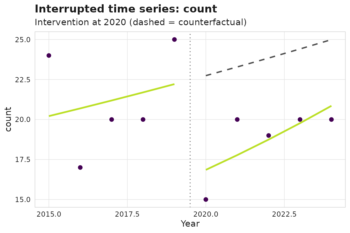
For citation-based outcomes, citation-immature recent years are excluded automatically (sm_citation_maturity() exposes the same flags on works).

A treated-vs-control comparison uses difference-in-differences. Here we tag two illustrative institution groups.

corpus$authorships$institution_name <- rep(
  c("Treated Inst", "Control Inst"),
  length.out = nrow(corpus$authorships))

did <- sm_did(corpus, treated = "Treated Inst", control = "Control Inst",
              intervention_year = 2020, outcome = "count")
did

4. Counting and robust impact

Fractional counting attributes a multi-author paper’s single unit of credit across its contributors.

head(sm_count(corpus, method = "fractional", level = "author"), 5)
#> # A tibble: 5 × 5
#>   entity_id  entity_name    n_works credit weighted_citations
#>   <chr>      <chr>            <int>  <dbl>              <dbl>
#> 1 A000000001 Raj Fischer         41  10.2               191. 
#> 2 A000000049 Mohammed Liu        16   4.79              103. 
#> 3 A000000060 Mohammed Kumar      13   4.68               64.3
#> 4 A000000070 Mei Mueller         13   4.38               91.3
#> 5 A000000041 Raj Andersson       11   4.16               79.9

Heavy-tailed metrics are summarised robustly with medians, bootstrap CIs, and the proportion of papers in the global top 10%.

sm_metric_summary(corpus, metric = "citations", seed = 1, n_boot = 500)
#> # A tibble: 1 × 8
#>   metric        n  mean median median_ci_low median_ci_high pp_top10 n_boot
#>   <chr>     <int> <dbl>  <dbl>         <dbl>          <dbl>    <dbl>  <int>
#> 1 citations   200  15.6     13            11           15.5      0.1    500

5. Reproducible reporting

Finally, sm_figure_manifest() turns a directory of exported figures into a captions / alt-text manifest for the manuscript.

dir <- withr::local_tempdir()
gg <- ggplot2::autoplot(its)
ggplot2::ggsave(file.path(dir, "fig_its.png"), gg, width = 6, height = 4,
                dpi = 150)
sm_figure_manifest(dir)
#> # A tibble: 1 × 6
#>   file        caption alt_text width height   dpi
#>   <chr>       <chr>   <chr>    <int>  <int> <dbl>
#> 1 fig_its.png ""      ""         900    600    59

Together these functions cover the recurring tasks of a research-coverage and impact study — audit, affiliation capture, policy evaluation, robust summarisation, and reporting — on top of the reproducible sm_corpus foundation.