Getting Started with songR

What is SONG?

SONG (Self-Organizing Nebulous Growths) is a parametric, incremental, noise-tolerant dimensionality reduction technique for data visualization. Unlike t-SNE and UMAP, SONG retains a parametric model that can be updated with new data without reinitializing the entire embedding. This makes SONG ideal for streaming data, incremental analysis, and noisy datasets.

The algorithm was developed by Senanayake et al. (2021) and published in IEEE Transactions on Neural Networks and Learning Systems. The songR package provides a native R/C++ implementation using RcppArmadillo.

Installation

# From CRAN (when available):
install.packages("songR")

# Development version from GitHub:
devtools::install_github("r-heller/songR")

Quick Start on Iris

The simplest way to use songR is the song() function, which fits a SONG model and returns an embedding:

library(songR)

model <- song(as.matrix(iris[, 1:4]),
              epochs = 10L,
              seed = 42,
              verbose = FALSE)

print(model)
#> SONG model
#>   Input: 150 points in 4 dimensions
#>   Coding vectors: 28 
#>   Edges: 49 
#>   Output dimensionality: 2 
#>   Epochs: 10 (max epochs)

The model contains the 2D embedding for all input points. Let’s visualize it:

plot(model, color_by = iris$Species)

Each color represents a different iris species. SONG discovers the natural cluster structure in the 4-dimensional data and maps it to 2D.

Bundled Dataset

songR ships with songR_blobs, a synthetic 8-cluster dataset in 20 dimensions designed for quick testing:

data(songR_blobs)
cat("Data:", nrow(songR_blobs$data), "x", ncol(songR_blobs$data), "\n")
#> Data: 1600 x 20
cat("Clusters:", length(unique(songR_blobs$labels)), "\n")
#> Clusters: 8

model_blobs <- song(songR_blobs$data,
                    epochs = 15L,
                    seed = 42,
                    verbose = FALSE)

plot(model_blobs, color_by = songR_blobs$labels)

Incremental Visualization

The key advantage of SONG is incremental updating. You can train on an initial batch of data and then add more data later without recomputing from scratch. The existing embedding is preserved.

# Split iris into two halves
X1 <- as.matrix(iris[1:75, 1:4])
X2 <- as.matrix(iris[76:150, 1:4])
labels1 <- iris$Species[1:75]
labels2 <- iris$Species[76:150]

# Fit on first half
model_v1 <- song(X1, epochs = 10L, seed = 42, verbose = FALSE)
emb_v1 <- model_v1$embedding
cat("After batch 1:", nrow(model_v1$C), "coding vectors\n")
#> After batch 1: 17 coding vectors

# Update with second half (NO reinit!)
model_v2 <- update(model_v1, X2, epochs = 10L, verbose = FALSE)
cat("After batch 2:", nrow(model_v2$C), "coding vectors\n")
#> After batch 2: 26 coding vectors

# Get embeddings for ALL points after update
emb_v2_all <- predict(model_v2, newdata = rbind(X1, X2))

Let’s see the before/after:

par(mfrow = c(1, 2), mar = c(2, 2, 3, 1))

# Before: only first 75 points
cols1 <- c(setosa = "#E41A1C", versicolor = "#377EB8",
           virginica = "#4DAF4A")[as.character(labels1)]
plot(emb_v1, pch = 16, col = cols1, cex = 0.8,
     main = "Step 1: First 75 points",
     xlab = "", ylab = "", bty = "n")

# After: all 150 points
cols_all <- c(setosa = "#E41A1C", versicolor = "#377EB8",
              virginica = "#4DAF4A")[as.character(iris$Species)]
plot(emb_v2_all, pch = 16, col = cols_all, cex = 0.8,
     main = "Step 2: All 150 points (incremental)",
     xlab = "", ylab = "", bty = "n")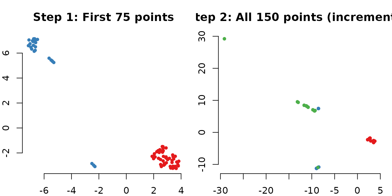

The first 75 points retain their approximate positions while the new data is smoothly integrated. This stability is measured by the CDY (Consecutive Displacement of Y) metric.

Projecting New Points

Once trained, a SONG model can project unseen data into the embedding space without retraining:

# Train on 80% of iris
train_idx <- sample(150, 120)
test_idx <- setdiff(1:150, train_idx)

model_train <- song(as.matrix(iris[train_idx, 1:4]),
                    epochs = 10L, seed = 42, verbose = FALSE)

# Project the held-out 20%
new_coords <- predict(model_train, newdata = as.matrix(iris[test_idx, 1:4]))

cat("Projected", nrow(new_coords), "new points into",
    ncol(new_coords), "dimensions\n")
#> Projected 30 new points into 2 dimensions

# Plot training points (circles) and projected points (triangles)
emb_train <- model_train$embedding

cols_train <- c(setosa = "#E41A1C", versicolor = "#377EB8",
                virginica = "#4DAF4A")[as.character(iris$Species[train_idx])]
cols_test <- c(setosa = "#E41A1C", versicolor = "#377EB8",
               virginica = "#4DAF4A")[as.character(iris$Species[test_idx])]

plot(rbind(emb_train, new_coords),
     pch = c(rep(16, nrow(emb_train)), rep(17, nrow(new_coords))),
     col = c(cols_train, cols_test),
     cex = c(rep(0.7, nrow(emb_train)), rep(1.2, nrow(new_coords))),
     main = "Training (circles) + Projected (triangles)",
     xlab = "SONG 1", ylab = "SONG 2", bty = "n")
legend("topright",
       legend = c("Training", "Projected"),
       pch = c(16, 17), bty = "n")

Model Inspection

summary(model_blobs)
#> SONG model summary
#> ==================
#>   Input: 1600 points in 20 dimensions
#>   Coding vectors: 136 
#>   Compression ratio: 11.8:1 
#>   Edges: 536 
#>   Mean edge strength: 0.6720 
#>   Output dimensionality: 2 
#>   Epochs: 15 (max epochs) 
#> 
#> Parameters:
#>   k = 3 | epsilon = 0.9 | spread_factor = 0.5 
#>   a = 1.577 | b = 0.895 | alpha = 1

Key Parameters

Parameter	Default	Effect
`epochs`	50	More epochs = better convergence, slower
`epsilon`	0.9	Edge decay: lower = sparser graph
`spread_factor`	0.5	Growth threshold: higher = more coding vectors
`k`	3	Neighborhood size for graph construction
`dispersion`	TRUE	UMAP refinement step for visual quality
`alpha`	1.0	Initial learning rate

When to Use SONG vs t-SNE vs UMAP

Feature	SONG	t-SNE	UMAP
Incremental updates	Yes	No	No
Parametric model	Yes	No	No
Noise tolerance	High	Low	Medium
Global structure	Good	Poor	Good
Speed (large data)	Medium	Slow	Fast
Best for	Streaming, incremental	Static, local detail	Static, fast overview

Citation

If you use songR in your research, please cite:

citation("songR")

Senanayake, D. A., Wang, W., Naik, S. H., & Halgamuge, S. (2021). Self-Organizing Nebulous Growths for Robust and Incremental Data Visualization. IEEE Transactions on Neural Networks and Learning Systems, 32(10), 4588-4602. doi:10.1109/TNNLS.2020.3023941

Session Info

sessionInfo()
#> R version 4.6.0 (2026-04-24)
#> Platform: x86_64-pc-linux-gnu
#> Running under: Ubuntu 24.04.4 LTS
#> 
#> Matrix products: default
#> BLAS:   /usr/lib/x86_64-linux-gnu/openblas-pthread/libblas.so.3 
#> LAPACK: /usr/lib/x86_64-linux-gnu/openblas-pthread/libopenblasp-r0.3.26.so;  LAPACK version 3.12.0
#> 
#> locale:
#>  [1] LC_CTYPE=C.UTF-8       LC_NUMERIC=C           LC_TIME=C.UTF-8       
#>  [4] LC_COLLATE=C.UTF-8     LC_MONETARY=C.UTF-8    LC_MESSAGES=C.UTF-8   
#>  [7] LC_PAPER=C.UTF-8       LC_NAME=C              LC_ADDRESS=C          
#> [10] LC_TELEPHONE=C         LC_MEASUREMENT=C.UTF-8 LC_IDENTIFICATION=C   
#> 
#> time zone: UTC
#> tzcode source: system (glibc)
#> 
#> attached base packages:
#> [1] stats     graphics  grDevices utils     datasets  methods   base     
#> 
#> other attached packages:
#> [1] songR_0.1.0
#> 
#> loaded via a namespace (and not attached):
#>  [1] vctrs_0.7.3        cli_3.6.6          knitr_1.51         rlang_1.2.0       
#>  [5] xfun_0.57          otel_0.2.0         S7_0.2.2           textshaping_1.0.5 
#>  [9] jsonlite_2.0.0     glue_1.8.1         htmltools_0.5.9    ragg_1.5.2        
#> [13] sass_0.4.10        uwot_0.2.4         scales_1.4.0       rmarkdown_2.31    
#> [17] grid_4.6.0         evaluate_1.0.5     jquerylib_0.1.4    fastmap_1.2.0     
#> [21] yaml_2.3.12        lifecycle_1.0.5    FNN_1.1.4.1        compiler_4.6.0    
#> [25] RColorBrewer_1.1-3 fs_2.1.0           Rcpp_1.1.1-1.1     lattice_0.22-9    
#> [29] farver_2.1.2       systemfonts_1.3.2  digest_0.6.39      R6_2.6.1          
#> [33] Matrix_1.7-5       bslib_0.10.0       gtable_0.3.6       tools_4.6.0       
#> [37] pkgdown_2.2.0      ggplot2_4.0.3      cachem_1.1.0       desc_1.4.3

Raban Heller

2026-05-04