library(tidyverse)
set.seed(42)
theme_set(theme_minimal(base_size = 12))Week 1, Session 1 — Scientific process and research workflow
Course 1 — #courses
Note
Workflow labs use the variant template: Goal → Approach → Execution → Check → Report.
Learning objectives
- Name the nine stages of the research workflow and say what goes wrong if each is skipped.
- Distinguish biological from statistical significance with an example.
- Frame a research question that can survive a methods section.
Prerequisites
R, RStudio, and Quarto installed (see Get started).
Background
Statistics is a thread running through a longer process that begins before a dataset exists. The research workflow — Question → Measurements → Design → Acquisition → Description → Analysis → Interpretation → Validation → Knowledge — names the stages of that process and makes clear that errors made at one stage are paid for at the next. A well-posed question protects you from a bad design; a good design protects you from a noisy dataset; a clean dataset protects you from needing exotic methods. Much of what looks like statistical failure in the literature is in fact a workflow failure three stages earlier.
The workflow also organises how you write up the work. The Introduction names the question; the Methods describe the measurements, design, and analysis; the Results describe the data and the inference; the Discussion interprets. When you plan an analysis in this order, the paper nearly writes itself. When you skip a stage, reviewers notice exactly which one.
Setup
1. Goal
Make the research workflow concrete by simulating a small clinical scenario and mapping each stage to a specific decision.
2. Approach
Imagine a new blood-pressure drug. Our simulated question: does drug X reduce systolic blood pressure compared with placebo in adults with hypertension? We will generate data that reflect a realistic effect and walk through the workflow.
n <- 120
df <- tibble(
  id    = seq_len(n),
  arm   = rep(c("placebo", "drug"), each = n / 2),
  sbp_0 = rnorm(n, mean = 150, sd = 10),
  sbp_1 = sbp_0 + ifelse(arm == "drug", -6, 0) + rnorm(n, 0, 8)
)
3. Execution
df |>
  mutate(delta = sbp_1 - sbp_0) |>
  ggplot(aes(arm, delta, fill = arm)) +
  geom_boxplot(alpha = 0.6, colour = "grey30") +
  labs(x = NULL, y = "Change in SBP (mmHg)") +
  theme(legend.position = "none")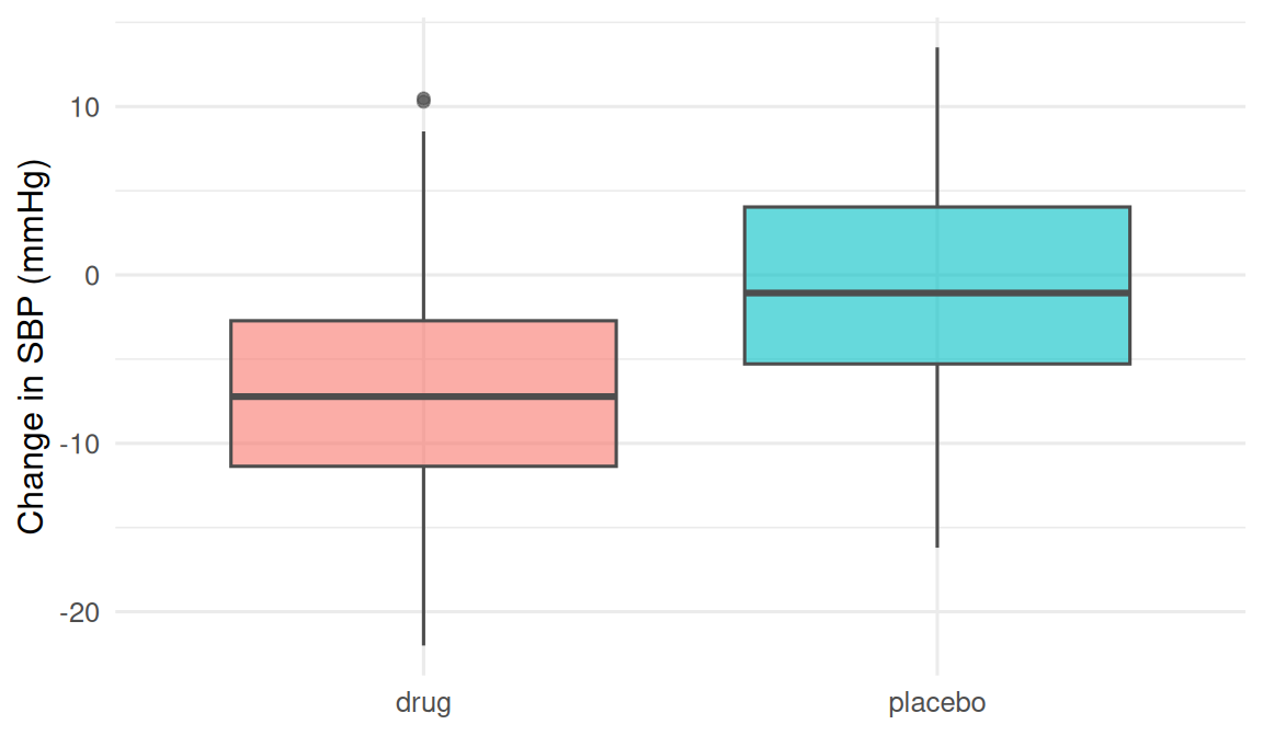
The plot is the Description stage. Without it, we would skip straight from raw numbers to a test. With it, the direction and spread of the change are visible before a single calculation.
4. Check
fit <- t.test(sbp_1 - sbp_0 ~ arm, data = df)
fit
    Welch Two Sample t-test

data:  sbp_1 - sbp_0 by arm
t = -4.1946, df = 117.89, p-value = 5.319e-05
alternative hypothesis: true difference in means between group drug and group placebo is not equal to 0
95 percent confidence interval:
 -8.062838 -2.891366
sample estimates:
   mean in group drug mean in group placebo
            -6.593619             -1.116518
The drug arm has a lower change-in-SBP on average; the interval is compatible with a clinically meaningful effect.
5. Report
In a simulated two-arm trial (n = 120), mean change in systolic blood pressure was 5.5 mmHg lower in the drug arm than in placebo (95% CI: -8.1 to -2.9; p = 5.3^{-5}).
Note the three pieces every report needs: direction and magnitude, an interval, and a p-value reported alongside — never instead of — the effect.
Biological vs statistical significance
A p-value below 0.05 does not, on its own, mean the effect matters clinically. A reduction of 0.1 mmHg in SBP would be statistically significant with a million patients but biologically meaningless. The discipline of asking how large is the effect? — not is there any effect? — is the single most important habit to form in Course 1.
Spend a minute on biological vs statistical significance during the presentation. Most reviewers catch this, most readers do not.
Common pitfalls
- Skipping the description stage and running a test on data you have never plotted.
- Reporting a p-value without an effect size and interval.
- Conflating biological and statistical significance.
- Treating the research workflow as optional once data are in hand.
Further reading
- Research workflow appendix.
- Altman DG. Practical Statistics for Medical Research, ch. 1.
- Wasserstein RL & Lazar NA (2016), The ASA’s Statement on p-Values.
Session info
sessionInfo()R version 4.5.2 (2025-10-31 ucrt)
Platform: x86_64-w64-mingw32/x64
Running under: Windows 11 x64 (build 26200)
Matrix products: default
LAPACK version 3.12.1
locale:
[1] LC_COLLATE=English_Germany.utf8 LC_CTYPE=English_Germany.utf8
[3] LC_MONETARY=English_Germany.utf8 LC_NUMERIC=C
[5] LC_TIME=English_Germany.utf8
time zone: Europe/Berlin
tzcode source: internal
attached base packages:
[1] stats graphics grDevices utils datasets methods base
other attached packages:
[1] lubridate_1.9.5 forcats_1.0.1 stringr_1.6.0 dplyr_1.2.1
[5] purrr_1.2.2 readr_2.2.0 tidyr_1.3.2 tibble_3.3.1
[9] ggplot2_4.0.3 tidyverse_2.0.0
loaded via a namespace (and not attached):
[1] gtable_0.3.6 jsonlite_2.0.0 compiler_4.5.2 tidyselect_1.2.1
[5] scales_1.4.0 yaml_2.3.12 fastmap_1.2.0 R6_2.6.1
[9] labeling_0.4.3 generics_0.1.4 knitr_1.51 htmlwidgets_1.6.4
[13] pillar_1.11.1 RColorBrewer_1.1-3 tzdb_0.5.0 rlang_1.2.0
[17] stringi_1.8.7 xfun_0.57 S7_0.2.2 otel_0.2.0
[21] timechange_0.4.0 cli_3.6.6 withr_3.0.2 magrittr_2.0.4
[25] digest_0.6.39 grid_4.5.2 hms_1.1.4 lifecycle_1.0.5
[29] vctrs_0.7.3 evaluate_1.0.5 glue_1.8.1 farver_2.1.2
[33] rmarkdown_2.31 tools_4.5.2 pkgconfig_2.0.3 htmltools_0.5.9