Week 2, Session 2 — Probability, conditional probability, Bayes’ theorem

Course 1 — #courses

Author

R. Heller

Note

Inference labs use the five-step template: Hypothesis → Visualise → Assumptions → Conduct → Conclude.

Learning objectives

Distinguish marginal, joint, and conditional probability and compute each from a contingency table.
State Bayes’ theorem and apply it to a medical-testing scenario.
Simulate a population and recover conditional probabilities by counting.

Prerequisites

Week 1.

Background

Probability is the language for reasoning under uncertainty. In biostatistics, most of the probabilities we care about are conditional — the probability that a patient has a disease given a test result; the probability of survival given a treatment; the probability of an adverse event given a risk factor. The distinction between marginal and conditional probability is the distinction between “how common is X in the population” and “how common is X in a particular subgroup”.

Bayes’ theorem is the rule for flipping a conditional probability. Given P(A|B) and the marginal probabilities P(A) and P(B), it returns P(B|A). In medical testing this lets us move from how often does the test fire when the disease is present (sensitivity) to how likely is disease given a positive test (positive predictive value). The two are routinely confused; Bayes’ theorem is the cure.

The counterintuitive part of Bayes is the role of prevalence. For a test with fixed sensitivity and specificity, PPV rises and falls with the prevalence in the tested population. Screening a very-low-risk population with an imperfect test guarantees that most positives will be false positives, regardless of the test’s quality.

Setup

library(tidyverse)
set.seed(42)
theme_set(theme_minimal(base_size = 12))

1. Hypothesis

We are not testing a hypothesis in the Fisherian sense; we are computing a conditional probability. The quantity of interest is the positive predictive value of a test with known sensitivity and specificity in a population of known prevalence.

2. Visualise

Simulate a population of 100,000 people. Prevalence of disease = 1%. Test sensitivity = 95%. Test specificity = 95%.

N <- 100000
prev <- 0.01
sens <- 0.95
spec <- 0.95

pop <- tibble(
  id = seq_len(N),
  disease = rbinom(N, 1, prev)
) |>
  mutate(
    test = if_else(disease == 1,
                   rbinom(N, 1, sens),
                   rbinom(N, 1, 1 - spec))
  )

tab <- table(disease = pop$disease, test = pop$test)
tab

       test
disease     0     1
      0 94154  4815
      1    43   988

as_tibble(tab) |>
  mutate(disease = recode(disease, `0` = "no disease", `1` = "disease"),
         test    = recode(test,    `0` = "neg", `1` = "pos")) |>
  ggplot(aes(test, disease, fill = n)) +
  geom_tile() +
  geom_text(aes(label = n), colour = "white") +
  scale_fill_viridis_c() +
  labs(x = "Test result", y = "True state", fill = "Count")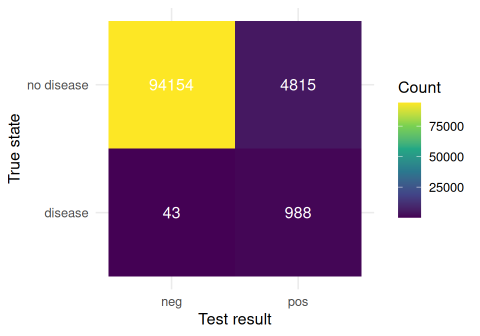

3. Assumptions

We assume each person is independent, the test’s operating characteristics are fixed, and no selection bias. Real screening has verification bias, spectrum bias, and imperfect gold standards; we are ignoring all of them to isolate the Bayesian calculation.

p_disease <- mean(pop$disease)
p_positive <- mean(pop$test)
p_pos_given_disease <- mean(pop$test[pop$disease == 1])
p_pos_given_no_disease <- mean(pop$test[pop$disease == 0])

tibble(quantity = c("P(D)", "P(T+)",
                    "P(T+|D)", "P(T+|~D)"),
       value = c(p_disease, p_positive,
                 p_pos_given_disease, p_pos_given_no_disease))

# A tibble: 4 × 2
  quantity  value
  <chr>     <dbl>
1 P(D)     0.0103
2 P(T+)    0.0580
3 P(T+|D)  0.958 
4 P(T+|~D) 0.0487

4. Conduct

Apply Bayes’ theorem by hand.

ppv_bayes <- (sens * prev) / (sens * prev + (1 - spec) * (1 - prev))
ppv_bayes

[1] 0.1610169

# By direct counting from the simulation.
ppv_count <- mean(pop$disease[pop$test == 1])
ppv_count

[1] 0.1702568

Same quantity, two routes. Bayes is algebra on the marginals; simulation is counting from the table. They must agree, within sampling error.

# Sweep prevalence from 0.001 to 0.5 and see PPV change.
sweep <- tibble(
  prev = seq(0.001, 0.5, length.out = 200),
  ppv = (sens * prev) / (sens * prev + (1 - spec) * (1 - prev))
)

sweep |>
  ggplot(aes(prev, ppv)) +
  geom_line(linewidth = 1) +
  geom_hline(yintercept = 0.5, linetype = 2, colour = "grey50") +
  labs(x = "Prevalence", y = "Positive predictive value")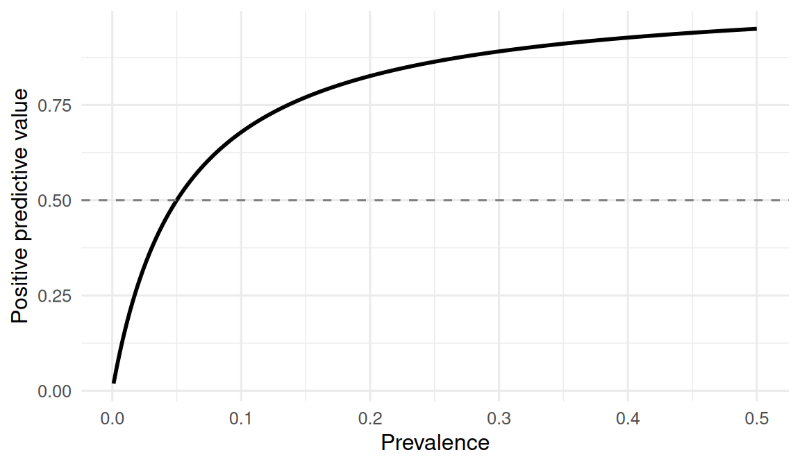

5. Concluding statement

With sensitivity = 0.95 and specificity = 0.95, a test applied in a population of prevalence = 0.01 has a positive predictive value of 0.161 — that is, fewer than one in five positive results is a true positive. In a simulated population of 1e+05, the PPV recovered by direct counting was 0.17. Negative predictive value was correspondingly high.

When prevalence is low, even a very accurate test produces mostly false positives. This is why population screening decisions are controversial, and why “my test is 95% accurate” is an incomplete statement.

Anchor this session in an example the audience will recognise — mammography, PSA, COVID rapid testing. The numbers are memorable.

Common pitfalls

Confusing sensitivity with PPV. P(T+|D) and P(D|T+) are not the same.
Reporting a test’s “accuracy” without specifying prevalence.
Assuming independence of repeated tests without checking.
Treating the prior (prevalence) as negotiable evidence.

Session info

sessionInfo()

R version 4.4.1 (2024-06-14)
Platform: x86_64-pc-linux-gnu
Running under: Ubuntu 24.04.4 LTS

Matrix products: default
BLAS:   /usr/lib/x86_64-linux-gnu/openblas-pthread/libblas.so.3 
LAPACK: /usr/lib/x86_64-linux-gnu/openblas-pthread/libopenblasp-r0.3.26.so;  LAPACK version 3.12.0

locale:
 [1] LC_CTYPE=C.UTF-8       LC_NUMERIC=C           LC_TIME=C.UTF-8       
 [4] LC_COLLATE=C.UTF-8     LC_MONETARY=C.UTF-8    LC_MESSAGES=C.UTF-8   
 [7] LC_PAPER=C.UTF-8       LC_NAME=C              LC_ADDRESS=C          
[10] LC_TELEPHONE=C         LC_MEASUREMENT=C.UTF-8 LC_IDENTIFICATION=C   

time zone: UTC
tzcode source: system (glibc)

attached base packages:
[1] stats     graphics  grDevices utils     datasets  methods   base     

other attached packages:
 [1] lubridate_1.9.5 forcats_1.0.1   stringr_1.6.0   dplyr_1.2.1    
 [5] purrr_1.2.2     readr_2.2.0     tidyr_1.3.2     tibble_3.3.1   
 [9] ggplot2_4.0.3   tidyverse_2.0.0

loaded via a namespace (and not attached):
 [1] gtable_0.3.6       jsonlite_2.0.0     compiler_4.4.1     tidyselect_1.2.1  
 [5] scales_1.4.0       yaml_2.3.12        fastmap_1.2.0      R6_2.6.1          
 [9] labeling_0.4.3     generics_0.1.4     knitr_1.51         htmlwidgets_1.6.4 
[13] pillar_1.11.1      RColorBrewer_1.1-3 tzdb_0.5.0         rlang_1.2.0       
[17] utf8_1.2.6         stringi_1.8.7      xfun_0.57          S7_0.2.2          
[21] otel_0.2.0         viridisLite_0.4.3  timechange_0.4.0   cli_3.6.6         
[25] withr_3.0.2        magrittr_2.0.5     digest_0.6.39      grid_4.4.1        
[29] hms_1.1.4          lifecycle_1.0.5    vctrs_0.7.3        evaluate_1.0.5    
[33] glue_1.8.1         farver_2.1.2       rmarkdown_2.31     tools_4.4.1       
[37] pkgconfig_2.0.3    htmltools_0.5.9

Learning objectives

Prerequisites

Background

Setup

1. Hypothesis

2. Visualise

3. Assumptions

4. Conduct

5. Concluding statement

Common pitfalls

Further reading

Session info

Related labs