library(tidyverse)
library(broom)
set.seed(42)
theme_set(theme_minimal(base_size = 12))Week 2, Session 5 — Non-linear regression with nls
Course 2 — #courses
Note
Inference labs use the five-step template: Hypothesis → Visualise → Assumptions → Conduct → Conclude.
Learning objectives
- Fit a parametric non-linear model with
nls()and report the three parameters. - Choose starting values that let the optimiser converge.
- Distinguish a GAM’s flexible curve from an
nlsmodel’s mechanistic curve.
Prerequisites
Sessions 2 and 4 of this week.
Background
Where a GAM says fit a smooth and see what shape it takes, nls says this curve has a known parametric form and I want the parameters. Michaelis–Menten kinetics, three-parameter logistic dose-response, and exponential decay are all examples of mechanistic models where the parameters have physical meanings: asymptote, half-maximal response, rate, and so on.
Fitting non-linear models is slightly more fragile than fitting linear ones because the optimiser must start somewhere and can get lost. Sensible starting values come from the shape of the data: the asymptote from the highest fitted values, the inflection from where the curve flattens, and so on. SSlogis and related self-starting functions estimate these automatically for common parameterisations.
nls gives asymptotic standard errors by default. For small samples or poor parameter identifiability, bootstrap or profile-likelihood intervals (confint(fit) uses profiles) are more honest.
Setup
1. Hypothesis
Simulate dose-response data and fit a three-parameter logistic.
2. Visualise
n <- 60
dose <- rep(c(0.1, 0.3, 1, 3, 10, 30), each = 10)
# true params: asym = 100, xmid = log(3), scal = 0.7 (log-scale)
true_resp <- 100 / (1 + exp(-(log(dose) - log(3)) / 0.7))
resp <- true_resp + rnorm(n, 0, 5)
dat <- tibble(dose, resp)

ggplot(dat, aes(dose, resp)) +
  geom_point(alpha = 0.7) +
  scale_x_log10() +
  labs(x = "Dose (log scale)", y = "Response")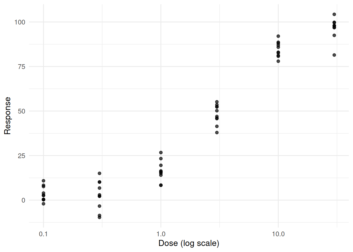
3. Assumptions
Correct model form, independent normal errors with constant variance on the response scale, and informative starting values.
fit <- nls(resp ~ SSlogis(log(dose), Asym, xmid, scal), data = dat)
resid_plot <- tibble(fitted = fitted(fit), resid = resid(fit))
ggplot(resid_plot, aes(fitted, resid)) +
  geom_point() +
  geom_hline(yintercept = 0, linetype = 2, colour = "grey50") +
  labs(x = "Fitted", y = "Residual")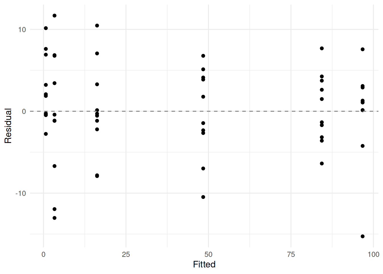
4. Conduct
summary(fit)
Formula: resp ~ SSlogis(log(dose), Asym, xmid, scal)

Parameters:
      Estimate Std. Error t value Pr(>|t|)
Asym 100.58109    2.60639   38.59   <2e-16 ***
xmid   1.15107    0.06694   17.20   <2e-16 ***
scal   0.69868    0.05199   13.44   <2e-16 ***
---
Signif. codes:  0 '***' 0.001 '**' 0.01 '*' 0.05 '.' 0.1 ' ' 1

Residual standard error: 5.799 on 57 degrees of freedom

Number of iterations to convergence: 0
Achieved convergence tolerance: 1.242e-07confint(fit) 2.5% 97.5%
Asym 95.7741920 106.3804894
xmid 1.0257176 1.2963776
scal 0.5989972 0.8113004pred <- tibble(dose = 10 ^ seq(-1, 1.5, length.out = 100))
pred$resp <- predict(fit, newdata = pred)
ggplot(dat, aes(dose, resp)) +
geom_point(alpha = 0.7) +
geom_line(data = pred, colour = "steelblue", linewidth = 0.8) +
scale_x_log10() +
labs(x = "Dose (log scale)", y = "Response")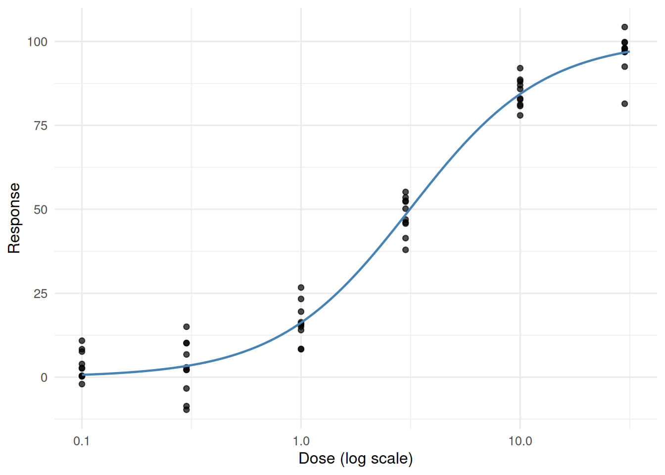
5. Concluding statement
A three-parameter logistic fitted on the log-dose scale returned an asymptote of 100.6 units and a mid-dose (EC50) at 3.16. Confidence intervals were obtained via the likelihood profile (see
confint).
Explain why the self-starting function matters: without it, the student is confronted with finding starts for three parameters from scratch, which distracts from the concept.
Common pitfalls
- Starting values that put the optimiser in a local minimum.
- Reporting symmetric SE-based intervals when the likelihood is asymmetric; prefer
confint. - Over-interpreting parameters when the data do not span the asymptote.
Further reading
- Bates DM, Watts DG. Nonlinear Regression Analysis and Its Applications.
- Ritz C, Streibig JC. Nonlinear Regression with R.
- Pinheiro JC, Bates DM. Mixed-Effects Models in S and S-PLUS, ch. 8.
Session info
sessionInfo()R version 4.5.2 (2025-10-31 ucrt)
Platform: x86_64-w64-mingw32/x64
Running under: Windows 11 x64 (build 26200)
Matrix products: default
LAPACK version 3.12.1
locale:
[1] LC_COLLATE=English_Germany.utf8 LC_CTYPE=English_Germany.utf8
[3] LC_MONETARY=English_Germany.utf8 LC_NUMERIC=C
[5] LC_TIME=English_Germany.utf8
time zone: Europe/Berlin
tzcode source: internal
attached base packages:
[1] stats graphics grDevices utils datasets methods base
other attached packages:
[1] broom_1.0.12 lubridate_1.9.5 forcats_1.0.1 stringr_1.6.0
[5] dplyr_1.2.1 purrr_1.2.2 readr_2.2.0 tidyr_1.3.2
[9] tibble_3.3.1 ggplot2_4.0.3 tidyverse_2.0.0
loaded via a namespace (and not attached):
[1] gtable_0.3.6 jsonlite_2.0.0 compiler_4.5.2 tidyselect_1.2.1
[5] scales_1.4.0 yaml_2.3.12 fastmap_1.2.0 R6_2.6.1
[9] labeling_0.4.3 generics_0.1.4 knitr_1.51 backports_1.5.1
[13] htmlwidgets_1.6.4 pillar_1.11.1 RColorBrewer_1.1-3 tzdb_0.5.0
[17] rlang_1.2.0 stringi_1.8.7 xfun_0.57 S7_0.2.2
[21] otel_0.2.0 timechange_0.4.0 cli_3.6.6 withr_3.0.2
[25] magrittr_2.0.4 digest_0.6.39 grid_4.5.2 hms_1.1.4
[29] lifecycle_1.0.5 vctrs_0.7.3 evaluate_1.0.5 glue_1.8.1
[33] farver_2.1.2 rmarkdown_2.31 tools_4.5.2 pkgconfig_2.0.3
[37] htmltools_0.5.9