library(tidyverse)
library(broom)
library(MASS)        # rlm; load before tidyverse dplyr::select is not needed here
library(sandwich)
library(lmtest)
set.seed(42)
theme_set(theme_minimal(base_size = 12))Week 1, Session 5 — Robust regression, weighted LS, HC (sandwich) standard errors
Course 2 — #courses
Note
Inference labs use the five-step template: Hypothesis → Visualise → Assumptions → Conduct → Conclude.
Learning objectives
- Fit a robust regression with
MASS::rlm()and compare coefficients with OLS. - Use weighted least squares when variance is known to vary with a predictor.
- Replace OLS standard errors with heteroscedasticity-consistent (sandwich) ones using
sandwich::vcovHCandlmtest::coeftest.
Prerequisites
Sessions 2–4 of this week.
Background
Classical OLS is optimal under a narrow set of assumptions. When residuals have heavy tails, a few observations can dominate the fit; M-estimators such as those in rlm downweight extreme residuals and return coefficients that reflect the bulk of the data. When variance is known to depend on a predictor, weighted least squares restores efficiency by weighting each observation by the inverse of its variance. When the variance pattern is unknown but you want valid inference, sandwich (HC) standard errors correct the standard errors without changing the point estimates.
The three tools solve different problems. Robust regression changes the coefficient. Weighted LS changes both the coefficient and the standard error if you have the correct weights. HC standard errors keep the OLS coefficient and replace only the standard errors. Choose the one that matches your threat.
The most common use of HC standard errors in practice is in cross-sectional regression where you suspect heteroscedasticity but have no good model for it. HC3 is a sensible default in small samples; HC0 is classical but liberal.
Setup
1. Hypothesis
Fit an OLS, a robust, and a weighted regression to the same data and compare. Then repeat the OLS with sandwich standard errors.
2. Visualise
n <- 200
x <- runif(n, 0, 10)
eps <- rnorm(n, 0, 0.3 + 0.2 * x)     # heteroscedastic
# a few extreme outliers
outl <- sample(seq_len(n), 8)
eps[outl] <- eps[outl] + rnorm(8, 0, 6)
y <- 2 + 0.7 * x + eps
dat <- tibble(x, y)

ggplot(dat, aes(x, y)) +
  geom_point(alpha = 0.6) +
  labs(x = "x", y = "y")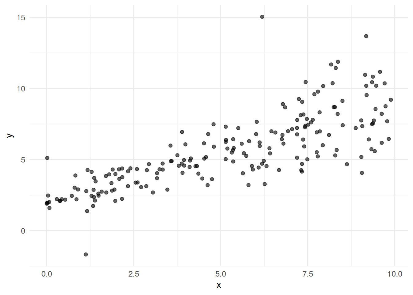
3. Assumptions
fit_ols <- lm(y ~ x, data = dat)
par(mfrow = c(2, 2))
plot(fit_ols)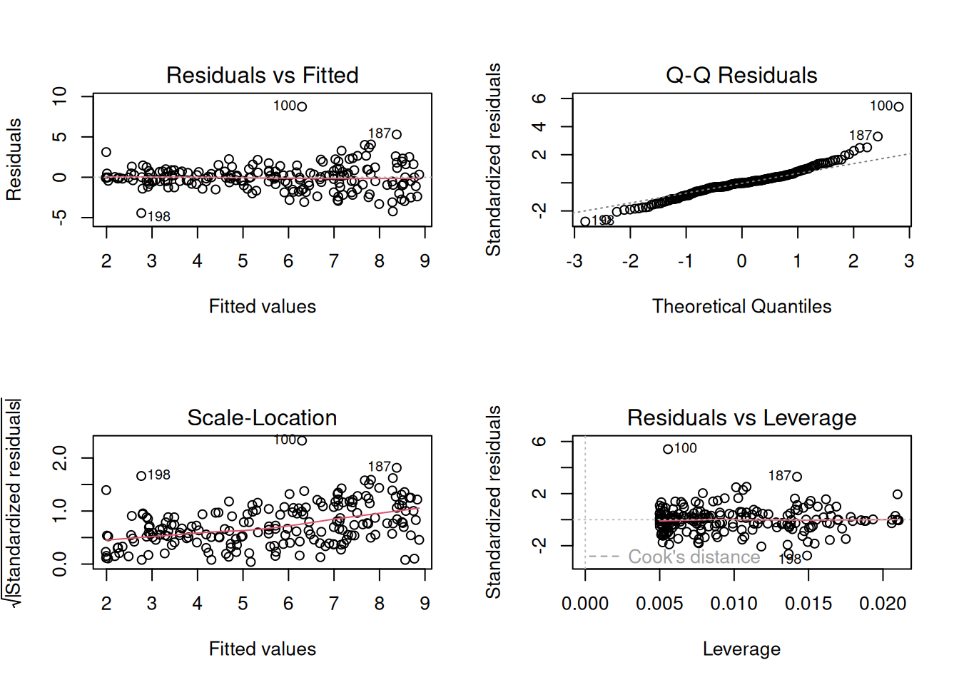
par(mfrow = c(1, 1))Fan-shaped residuals and heavy QQ tails — textbook cue for robust or sandwich treatment.
4. Conduct
OLS, robust, and weighted fits:
fit_rlm <- MASS::rlm(y ~ x, data = dat)
# variance grows roughly with x; weight by 1 / (fitted variance proxy)
w <- 1 / (0.3 + 0.2 * dat$x)^2
fit_wls <- lm(y ~ x, data = dat, weights = w)

bind_rows(
  tidy(fit_ols) |> mutate(model = "OLS"),
  tibble(term = c("(Intercept)", "x"),
         estimate = coef(fit_rlm),
         std.error = sqrt(diag(vcov(fit_rlm))),
         model = "robust"),
  tidy(fit_wls) |> mutate(model = "WLS")
) |>
  filter(term == "x") |>
  dplyr::select(model, estimate, std.error)
# A tibble: 3 × 3
model estimate std.error
<chr> <dbl> <dbl>
1 OLS 0.697 0.0393
2 robust 0.680 0.0336
3 WLS 0.665 0.0362Sandwich SEs on the OLS fit:
coeftest(fit_ols, vcov. = vcovHC(fit_ols, type = "HC3"))
t test of coefficients:

            Estimate Std. Error t value  Pr(>|t|)
(Intercept) 1.981555   0.172748  11.471 < 2.2e-16 ***
x           0.696813   0.039644  17.577 < 2.2e-16 ***
---
Signif. codes:  0 '***' 0.001 '**' 0.01 '*' 0.05 '.' 0.1 ' ' 1
5. Concluding statement
OLS, robust, and weighted fits gave similar slope estimates (approximately 0.7, 0.68, and 0.66 respectively). Classical OLS standard errors were biased by heteroscedasticity; HC3 sandwich standard errors were preferred for inference.
The three methods are complements, not substitutes. Teach the decision tree: outliers → robust; known variance pattern → weighted; unknown variance pattern → sandwich.
Common pitfalls
- Using
rlmand then testing coefficients with classical OLS code that does not know the residuals were reweighted. - Choosing weights from the residuals of an earlier fit without acknowledging the circularity.
- Quoting HC standard errors without saying which HC flavour was used.
Further reading
- Huber PJ, Ronchetti EM. Robust Statistics, 2nd ed.
- MacKinnon JG, White H (1985), Some heteroscedasticity-consistent…
- Zeileis A (2004), Econometric computing with HC and HAC errors.
Session info
sessionInfo()R version 4.5.2 (2025-10-31 ucrt)
Platform: x86_64-w64-mingw32/x64
Running under: Windows 11 x64 (build 26200)
Matrix products: default
LAPACK version 3.12.1
locale:
[1] LC_COLLATE=English_Germany.utf8 LC_CTYPE=English_Germany.utf8
[3] LC_MONETARY=English_Germany.utf8 LC_NUMERIC=C
[5] LC_TIME=English_Germany.utf8
time zone: Europe/Berlin
tzcode source: internal
attached base packages:
[1] stats graphics grDevices utils datasets methods base
other attached packages:
[1] lmtest_0.9-40 zoo_1.8-15 sandwich_3.1-1 MASS_7.3-65
[5] broom_1.0.12 lubridate_1.9.5 forcats_1.0.1 stringr_1.6.0
[9] dplyr_1.2.1 purrr_1.2.2 readr_2.2.0 tidyr_1.3.2
[13] tibble_3.3.1 ggplot2_4.0.3 tidyverse_2.0.0
loaded via a namespace (and not attached):
[1] gtable_0.3.6 jsonlite_2.0.0 compiler_4.5.2 tidyselect_1.2.1
[5] scales_1.4.0 yaml_2.3.12 fastmap_1.2.0 lattice_0.22-9
[9] R6_2.6.1 labeling_0.4.3 generics_0.1.4 knitr_1.51
[13] backports_1.5.1 htmlwidgets_1.6.4 pillar_1.11.1 RColorBrewer_1.1-3
[17] tzdb_0.5.0 rlang_1.2.0 utf8_1.2.6 stringi_1.8.7
[21] xfun_0.57 S7_0.2.2 otel_0.2.0 timechange_0.4.0
[25] cli_3.6.6 withr_3.0.2 magrittr_2.0.4 digest_0.6.39
[29] grid_4.5.2 hms_1.1.4 lifecycle_1.0.5 vctrs_0.7.3
[33] evaluate_1.0.5 glue_1.8.1 farver_2.1.2 rmarkdown_2.31
[37] tools_4.5.2 pkgconfig_2.0.3 htmltools_0.5.9