library(tidyverse)
library(broom)
library(MASS)
set.seed(42)
theme_set(theme_minimal(base_size = 12))Week 3, Session 4 — Poisson and negative-binomial regression
Course 2 — #courses
Note
Inference labs use the five-step template: Hypothesis → Visualise → Assumptions → Conduct → Conclude.
Learning objectives
- Fit a Poisson GLM for counts with
glm(family = poisson)and use an offset for exposure. - Diagnose overdispersion and switch to negative-binomial regression with
MASS::glm.nbwhen needed. - Report incidence rate ratios with intervals.
Prerequisites
Week 3 Session 1 on logistic regression.
Background
Counts with a known exposure are the natural habitat of the Poisson GLM: number of events per person-year, per square metre, per trap night. The canonical link is the log, so the exponentiated coefficient is an incidence rate ratio. Exposure enters the model as an offset — a term with a fixed coefficient of 1 on the log scale.
The Poisson model assumes variance equals the mean. Most real count data violate this, with variance growing faster than the mean. Overdispersion inflates Type-I error when ignored. Checking the ratio of residual deviance to its degrees of freedom gives a quick read; when it is substantially above 1, the negative-binomial GLM (or a quasi-Poisson variance) is a better fit.
Poisson regression without an offset is a common trap. If the denominators vary, a coefficient on an exposure variable is confounded with exposure; the offset separates the two and restores the interpretation of the log-rate ratio.
Setup
1. Hypothesis
Simulate counts of events with a dispersion parameter larger than 1 (so negative-binomial is the correct model), plus a known exposure.
2. Visualise
n <- 300
x <- rnorm(n)
exposure <- runif(n, 0.5, 2)
mu <- exposure * exp(0.5 + 0.4 * x)
# negative-binomial counts with theta = 2 (overdispersion)
y <- rnegbin(n, mu = mu, theta = 2)
dat <- tibble(x, exposure, y)

ggplot(dat, aes(x, y)) +
  geom_point(alpha = 0.6) +
  labs(x = "x", y = "Count")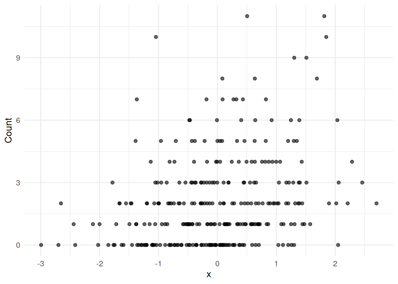
3. Assumptions
Independent counts; correct mean structure; for Poisson, variance = mean.
fit_p <- glm(y ~ x + offset(log(exposure)), data = dat, family = poisson)
# dispersion
dev_over_df <- deviance(fit_p) / df.residual(fit_p)
dev_over_df
[1] 1.918715Dispersion >> 1 signals negative-binomial.
4. Conduct
fit_nb <- glm.nb(y ~ x + offset(log(exposure)), data = dat)

bind_rows(
  tidy(fit_p, conf.int = TRUE, exponentiate = TRUE) |> mutate(model = "Poisson"),
  tidy(fit_nb, conf.int = TRUE, exponentiate = TRUE) |> mutate(model = "NB")
) |>
  filter(term == "x") |>
  dplyr::select(model, estimate, conf.low, conf.high, std.error)
# A tibble: 2 × 5
model estimate conf.low conf.high std.error
<chr> <dbl> <dbl> <dbl> <dbl>
1 Poisson 1.35 1.25 1.47 0.0416
2 NB 1.35 1.21 1.52 0.0579The estimates are similar but the NB standard error is larger and honest.
5. Concluding statement
Event counts increased with x (NB IRR per unit x = 1.35; 95% CI 1.21 to 1.52). Poisson residual deviance indicated overdispersion; we therefore report the negative-binomial fit as primary.
Encourage students to always fit both and report the NB when dispersion is above 1.2 or so; it will very rarely hurt.
Common pitfalls
- Forgetting the offset when denominators vary.
- Using Poisson when overdispersion is present.
- Reporting the rate ratio without an interval.
Further reading
- McCullagh P, Nelder JA. Generalized Linear Models, ch. 6.
- Hilbe JM. Negative Binomial Regression.
- Zeileis A, Kleiber C, Jackman S (2008), Regression models for count data.
Session info
sessionInfo()R version 4.5.2 (2025-10-31 ucrt)
Platform: x86_64-w64-mingw32/x64
Running under: Windows 11 x64 (build 26200)
Matrix products: default
LAPACK version 3.12.1
locale:
[1] LC_COLLATE=English_Germany.utf8 LC_CTYPE=English_Germany.utf8
[3] LC_MONETARY=English_Germany.utf8 LC_NUMERIC=C
[5] LC_TIME=English_Germany.utf8
time zone: Europe/Berlin
tzcode source: internal
attached base packages:
[1] stats graphics grDevices utils datasets methods base
other attached packages:
[1] MASS_7.3-65 broom_1.0.12 lubridate_1.9.5 forcats_1.0.1
[5] stringr_1.6.0 dplyr_1.2.1 purrr_1.2.2 readr_2.2.0
[9] tidyr_1.3.2 tibble_3.3.1 ggplot2_4.0.3 tidyverse_2.0.0
loaded via a namespace (and not attached):
[1] gtable_0.3.6 jsonlite_2.0.0 compiler_4.5.2 tidyselect_1.2.1
[5] scales_1.4.0 yaml_2.3.12 fastmap_1.2.0 R6_2.6.1
[9] labeling_0.4.3 generics_0.1.4 knitr_1.51 backports_1.5.1
[13] htmlwidgets_1.6.4 pillar_1.11.1 RColorBrewer_1.1-3 tzdb_0.5.0
[17] rlang_1.2.0 utf8_1.2.6 stringi_1.8.7 xfun_0.57
[21] S7_0.2.2 otel_0.2.0 timechange_0.4.0 cli_3.6.6
[25] withr_3.0.2 magrittr_2.0.4 digest_0.6.39 grid_4.5.2
[29] hms_1.1.4 lifecycle_1.0.5 vctrs_0.7.3 evaluate_1.0.5
[33] glue_1.8.1 farver_2.1.2 rmarkdown_2.31 tools_4.5.2
[37] pkgconfig_2.0.3 htmltools_0.5.9