library(tidyverse)
library(broom)
library(MASS)
set.seed(42)
theme_set(theme_minimal(base_size = 12))Week 3, Session 1 — Logistic regression (binomial GLM)
Course 2 — #courses
Note
Inference labs use the five-step template: Hypothesis → Visualise → Assumptions → Conduct → Conclude.
Learning objectives
- Fit a logistic regression with
glm(family = binomial)and translate coefficients into odds ratios. - Construct a confusion matrix at a chosen probability threshold.
- Report the model with an odds ratio, an interval, and a brief note on discrimination.
Prerequisites
Week 1 regression material.
Background
Logistic regression models the log-odds of a binary outcome as a linear combination of predictors. The exponent of a coefficient is the odds ratio for a one-unit increase in the corresponding predictor. Because the relationship is linear on the log-odds scale and not the probability scale, a slope of 0.5 log-odds is a larger change in probability near 0.5 than near 0.95.
The model is fit by maximum likelihood with iteratively reweighted least squares. Standard errors are computed from the observed information, and Wald intervals on the log-odds scale are exponentiated to give intervals on the odds ratio. Profile-likelihood intervals are more trustworthy when the sample is small or the predictor is strongly associated with the outcome.
A confusion matrix at a single threshold tells only part of the story; the thresholds used in the clinic may not be the one that maximises accuracy. Week 3, Session 5 covers ROC curves and calibration, which give a threshold-free view of the same model.
Setup
1. Hypothesis
Using MASS::Pima.tr, can plasma glucose (glu) predict diabetes status (type)?
2. Visualise
pima <- as_tibble(Pima.tr) |>
  mutate(type = factor(type, levels = c("No", "Yes")))

ggplot(pima, aes(type, glu, fill = type)) +
  geom_boxplot(alpha = 0.6, colour = "grey30") +
  labs(x = "Diabetes", y = "Plasma glucose") +
  theme(legend.position = "none")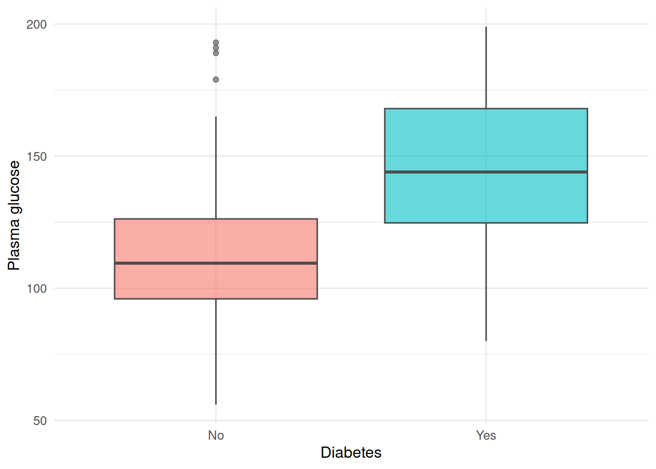
3. Assumptions
Binary outcome, independent observations, log-odds linear in the predictors (or handled explicitly with a smooth/transformation).
fit <- glm(type ~ glu, data = pima, family = binomial)
# residuals are less informative in GLMs; check for linearity on the logit scale
pima |>
  mutate(p = fitted(fit),
         logit = qlogis(p)) |>
  ggplot(aes(glu, logit)) +
  geom_point(alpha = 0.5) +
  geom_smooth(method = "loess", se = FALSE, colour = "steelblue") +
  labs(x = "Plasma glucose", y = "Fitted logit")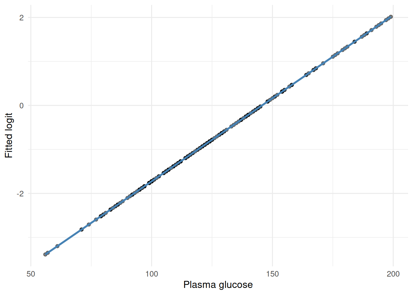
4. Conduct
tidy(fit, conf.int = TRUE, exponentiate = TRUE)# A tibble: 2 × 7
term estimate std.error statistic p.value conf.low conf.high
<chr> <dbl> <dbl> <dbl> <dbl> <dbl> <dbl>
1 (Intercept) 0.00407 0.836 -6.58 4.62e-11 0.000714 0.0192
2 glu 1.04 0.00628 6.02 1.76e- 9 1.03 1.05 glance(fit)# A tibble: 1 × 8
null.deviance df.null logLik AIC BIC deviance df.residual nobs
<dbl> <int> <dbl> <dbl> <dbl> <dbl> <int> <int>
1 256. 199 -104. 211. 218. 207. 198 200pred_prob <- predict(fit, type = "response")
pred_class <- ifelse(pred_prob > 0.5, "Yes", "No")
table(pred_class, truth = pima$type) truth
pred_class No Yes
No 118 36
Yes 14 325. Concluding statement
In 200 women, each 10 mg/dL increase in plasma glucose was associated with an odds ratio for diabetes of 1.46 (95% CI from profile: 1.3 to 1.66). At a 0.5 threshold the classifier had 75% accuracy; a threshold-free assessment appears in Week 3 Session 5.
Most readers prefer ORs reported per 10 units of a continuous predictor rather than per single unit; the per-unit OR sometimes looks implausibly close to 1.
Common pitfalls
- Reporting the coefficient on the log-odds scale without exponentiating.
- Confusing probability and odds.
- Evaluating the model with accuracy at one threshold and nothing else.
Further reading
- Hosmer DW, Lemeshow S. Applied Logistic Regression.
- Harrell FE. Regression Modeling Strategies, ch. 10.
- Gelman A, Hill J. Data Analysis Using Regression and Multilevel….
Session info
sessionInfo()R version 4.5.2 (2025-10-31 ucrt)
Platform: x86_64-w64-mingw32/x64
Running under: Windows 11 x64 (build 26200)
Matrix products: default
LAPACK version 3.12.1
locale:
[1] LC_COLLATE=English_Germany.utf8 LC_CTYPE=English_Germany.utf8
[3] LC_MONETARY=English_Germany.utf8 LC_NUMERIC=C
[5] LC_TIME=English_Germany.utf8
time zone: Europe/Berlin
tzcode source: internal
attached base packages:
[1] stats graphics grDevices utils datasets methods base
other attached packages:
[1] MASS_7.3-65 broom_1.0.12 lubridate_1.9.5 forcats_1.0.1
[5] stringr_1.6.0 dplyr_1.2.1 purrr_1.2.2 readr_2.2.0
[9] tidyr_1.3.2 tibble_3.3.1 ggplot2_4.0.3 tidyverse_2.0.0
loaded via a namespace (and not attached):
[1] Matrix_1.7-5 gtable_0.3.6 jsonlite_2.0.0 compiler_4.5.2
[5] tidyselect_1.2.1 splines_4.5.2 scales_1.4.0 yaml_2.3.12
[9] fastmap_1.2.0 lattice_0.22-9 R6_2.6.1 labeling_0.4.3
[13] generics_0.1.4 knitr_1.51 backports_1.5.1 htmlwidgets_1.6.4
[17] pillar_1.11.1 RColorBrewer_1.1-3 tzdb_0.5.0 rlang_1.2.0
[21] utf8_1.2.6 stringi_1.8.7 xfun_0.57 S7_0.2.2
[25] otel_0.2.0 timechange_0.4.0 cli_3.6.6 mgcv_1.9-4
[29] withr_3.0.2 magrittr_2.0.4 digest_0.6.39 grid_4.5.2
[33] hms_1.1.4 nlme_3.1-169 lifecycle_1.0.5 vctrs_0.7.3
[37] evaluate_1.0.5 glue_1.8.1 farver_2.1.2 rmarkdown_2.31
[41] tools_4.5.2 pkgconfig_2.0.3 htmltools_0.5.9