library(tidyverse)
library(gtsummary)
library(broom)
library(palmerpenguins)
set.seed(42)
theme_set(theme_minimal(base_size = 12))Week 4, Session 5 — Explanation vs prediction; reporting
Course 2 — #courses
Note
Workflow lab: Goal → Approach → Execution → Check → Report.
Learning objectives
- Distinguish explanatory from predictive modelling, and choose the correct evaluation metric for each.
- Map STROBE, TRIPOD, STARD, and CONSORT onto the study designs each is meant for.
- Produce a publication-ready regression table with
gtsummarywhose numbers trace directly to the fitted model.
Prerequisites
The regression tools covered across Course 2.
Background
Breiman’s 1998 essay The Two Cultures and Shmueli’s 2010 essay To Explain or to Predict? draw the same line from opposite sides. In explanatory modelling the goal is inference — what is the estimated effect of X on Y, adjusted for confounders? — and the right evaluation metric is bias-unbiasedness, interval coverage, and interpretability. In predictive modelling the goal is accuracy on unseen data, and the right evaluation metric is out-of-sample loss, calibration, and decision utility. The statistical machinery overlaps but the habits around it do not; a regression that makes an excellent explanation often makes a lacklustre prediction, and vice versa.
Reporting guidelines are the mechanism by which the field enforces discipline around these two cultures. STROBE for observational studies, CONSORT for randomised trials, STARD for diagnostic accuracy, and TRIPOD (now TRIPOD-AI) for prediction models each specify the items a reader needs to evaluate the claim. A checklist filled in as you write is much easier than one filled in at submission.
Setup
1. Goal
Fit a single linear model to the penguins data and present it two ways: once as an explanatory analysis (what drives body mass?) and once as a predictive model (can we predict body mass on held-out birds?).
2. Approach
peng <- penguins |> drop_na(body_mass_g, flipper_length_mm, sex, species)
fit_expl <- lm(body_mass_g ~ flipper_length_mm + sex + species, data = peng)
3. Execution
peng |>
  ggplot(aes(flipper_length_mm, body_mass_g, colour = species)) +
  geom_point(alpha = 0.6) +
  geom_smooth(method = "lm", se = FALSE, linewidth = 0.8) +
  labs(x = "Flipper length (mm)", y = "Body mass (g)")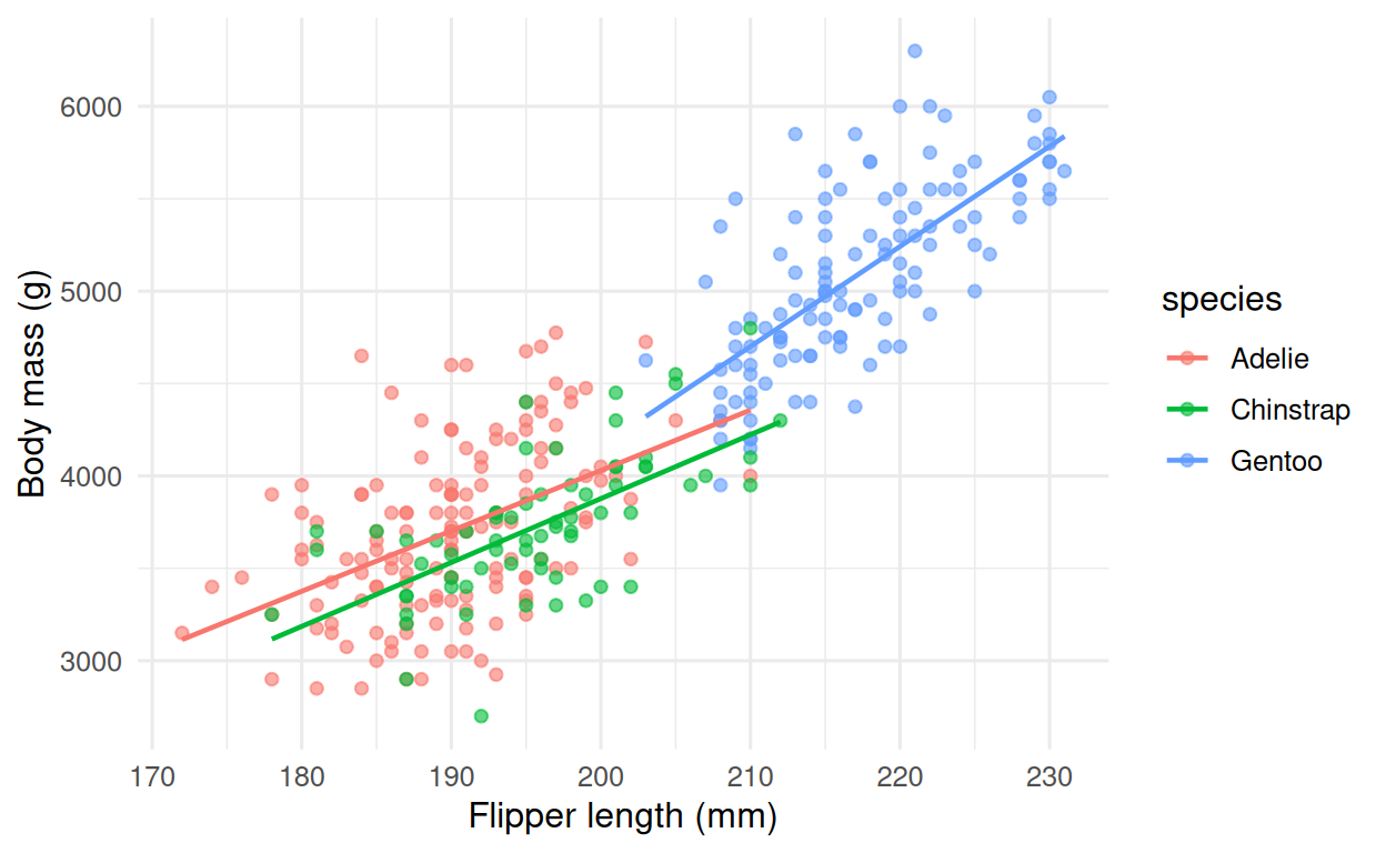
4. Check
Explanatory evaluation: effect sizes with intervals, residual diagnostics, and adjusted R².
glance(fit_expl) |> select(r.squared, adj.r.squared, sigma, df, df.residual)# A tibble: 1 × 5
r.squared adj.r.squared sigma df df.residual
<dbl> <dbl> <dbl> <dbl> <int>
1 0.867 0.865 296. 4 328Predictive evaluation: a 5-fold split, hand-coded to keep the example transparent.
k <- 5
folds <- sample(rep(seq_len(k), length.out = nrow(peng)))
rmse_k <- sapply(seq_len(k), function(i) {
  tr <- peng[folds != i, ]
  te <- peng[folds == i, ]
  f  <- lm(body_mass_g ~ flipper_length_mm + sex + species, data = tr)
  sqrt(mean((predict(f, te) - te$body_mass_g)^2))
})
mean_rmse <- mean(rmse_k)
mean_rmse
[1] 294.96555. Report
tbl_regression(fit_expl, intercept = TRUE) |>
modify_caption("**Table 1. Linear-regression estimates for body mass (g).**")| Characteristic | Beta | 95% CI | p-value |
|---|---|---|---|
| (Intercept) | -366 | -1,412, 681 | 0.5 |
| flipper_length_mm | 20 | 14, 26 | <0.001 |
| sex | |||
| female | — | — | |
| male | 530 | 456, 605 | <0.001 |
| species | |||
| Adelie | — | — | |
| Chinstrap | -88 | -179, 3.5 | 0.060 |
| Gentoo | 836 | 669, 1,004 | <0.001 |
| Abbreviation: CI = Confidence Interval | |||
In the Palmer penguins dataset (n = 333), body mass was associated with flipper length, sex, and species (adjusted R² = 0.87). Out-of-sample performance, estimated by 5-fold cross-validation, was RMSE = 295 g.
Reporting-guideline map
| Design | Guideline | URL |
|---|---|---|
| Randomised trial | CONSORT | https://www.consort-statement.org/ |
| Observational study | STROBE | https://www.strobe-statement.org/ |
| Diagnostic-accuracy study | STARD | https://www.equator-network.org/reporting-guidelines/stard/ |
| Prediction-model study | TRIPOD / TRIPOD-AI | https://www.tripod-statement.org/ |
| Systematic review | PRISMA | http://prisma-statement.org/ |
The distinction to impress on a PhD audience: an effect size in an explanatory model is an answer to a scientific question; in a predictive model it is an implementation detail.
Common pitfalls
- Choosing a predictor set by R² and reporting a predictive claim, or tuning a predictive model and reporting causal-sounding coefficients.
- Filling in a reporting checklist at submission rather than while drafting.
- Assuming in-sample R² generalises.
Further reading
- Breiman L. (2001). Statistical Modeling: The Two Cultures.
- Shmueli G. (2010). To Explain or to Predict? Statistical Science.
- Writing a report.
Session info
sessionInfo()R version 4.5.2 (2025-10-31 ucrt)
Platform: x86_64-w64-mingw32/x64
Running under: Windows 11 x64 (build 26200)
Matrix products: default
LAPACK version 3.12.1
locale:
[1] LC_COLLATE=English_Germany.utf8 LC_CTYPE=English_Germany.utf8
[3] LC_MONETARY=English_Germany.utf8 LC_NUMERIC=C
[5] LC_TIME=English_Germany.utf8
time zone: Europe/Berlin
tzcode source: internal
attached base packages:
[1] stats graphics grDevices utils datasets methods base
other attached packages:
[1] palmerpenguins_0.1.1 broom_1.0.12 gtsummary_2.5.0
[4] lubridate_1.9.5 forcats_1.0.1 stringr_1.6.0
[7] dplyr_1.2.1 purrr_1.2.2 readr_2.2.0
[10] tidyr_1.3.2 tibble_3.3.1 ggplot2_4.0.3
[13] tidyverse_2.0.0
loaded via a namespace (and not attached):
[1] gt_1.3.0 sass_0.4.10 generics_0.1.4
[4] xml2_1.5.2 stringi_1.8.7 lattice_0.22-9
[7] hms_1.1.4 digest_0.6.39 magrittr_2.0.4
[10] evaluate_1.0.5 grid_4.5.2 timechange_0.4.0
[13] RColorBrewer_1.1-3 cards_0.7.1 fastmap_1.2.0
[16] broom.helpers_1.22.0 jsonlite_2.0.0 Matrix_1.7-5
[19] backports_1.5.1 mgcv_1.9-4 scales_1.4.0
[22] labelled_2.16.0 cli_3.6.6 rlang_1.2.0
[25] litedown_0.9 commonmark_2.0.0 splines_4.5.2
[28] base64enc_0.1-6 withr_3.0.2 yaml_2.3.12
[31] otel_0.2.0 tools_4.5.2 tzdb_0.5.0
[34] vctrs_0.7.3 R6_2.6.1 lifecycle_1.0.5
[37] fs_2.1.0 htmlwidgets_1.6.4 pkgconfig_2.0.3
[40] pillar_1.11.1 gtable_0.3.6 glue_1.8.1
[43] haven_2.5.5 xfun_0.57 tidyselect_1.2.1
[46] knitr_1.51 farver_2.1.2 htmltools_0.5.9
[49] nlme_3.1-169 rmarkdown_2.31 labeling_0.4.3
[52] compiler_4.5.2 S7_0.2.2 markdown_2.0