library(tidyverse)
set.seed(42)
theme_set(theme_minimal(base_size = 12))Week 1, Session 3 — Adaptive, non-inferiority, equivalence trials
Course 3 — #courses
Note
Inference lab using the five-step template: Hypothesis → Visualise → Assumptions → Conduct → Conclude.
Learning objectives
- Distinguish superiority, non-inferiority, and equivalence trials by their null hypotheses.
- Choose a non-inferiority margin and say what it means clinically.
- Run and plot a non-inferiority test with a confidence interval versus the margin.
Prerequisites
Course 1 inference and Course 2 confidence intervals.
Background
A superiority trial asks whether a new treatment beats the comparator. A non-inferiority (NI) trial asks whether the new treatment is not worse than the comparator by more than a pre-specified margin (often called Δ). An equivalence trial asks whether the new treatment is neither better nor worse than the comparator by more than Δ on either side. These are distinct statistical questions and they require different designs, analyses, and sample sizes.
The NI margin is the hardest thing about an NI trial. It has to be small enough that clinicians and patients would trade it for the benefits of the new treatment (lower cost, fewer side effects, easier administration), but not so small that the trial is infeasible. Regulators will often ask for a margin no larger than a defined fraction of the historical treatment effect of the comparator versus placebo.
Adaptive trials modify some aspect of the design (sample size, arm allocation, the decision rule) during the trial based on interim results, using pre-specified rules. Group sequential designs, for example, stop early for overwhelming efficacy or for futility, while spending Type I error according to a chosen alpha-spending function.
A one-sided 97.5% confidence interval that stays on the correct side of the margin is the operational test in most NI trials. Graphically, this is a forest plot where you check that the interval does not cross the margin line.
Setup
1. Hypothesis
H0: the new treatment is worse than the comparator by more than Δ = 3 units on a continuous outcome. H1: the new treatment is not worse by more than Δ.
2. Visualise
n <- 150
trial <- tibble(
  arm = rep(c("comparator", "new"), each = n),
  y   = c(rnorm(n, 70, 10), rnorm(n, 69, 10))
)

trial |>
  ggplot(aes(arm, y, fill = arm)) +
  geom_boxplot(alpha = 0.6, colour = "grey30") +
  labs(x = NULL, y = "Outcome") +
  theme(legend.position = "none")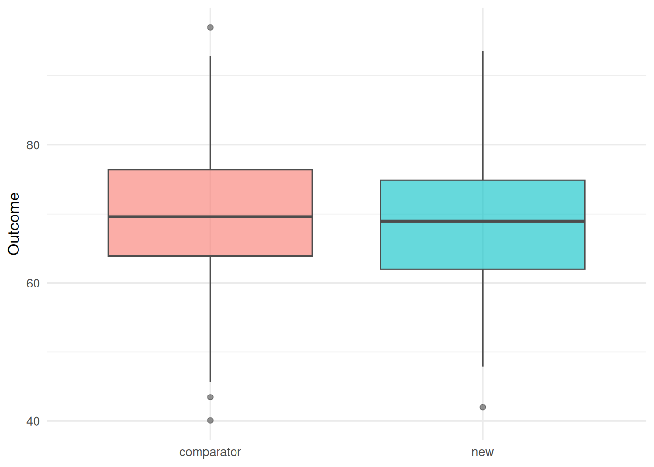
3. Assumptions
Independent observations, roughly normal within-arm residuals, and a pre-specified margin declared before looking at the data. The direction of the test matters: we test whether the lower bound of the mean difference (new − comparator) is above −Δ.
4. Conduct
fit <- t.test(y ~ arm, data = trial)
fit
    Welch Two Sample t-test

data:  y by arm
t = 0.75382, df = 297.66, p-value = 0.4516
alternative hypothesis: true difference in means between group comparator and group new is not equal to 0
95 percent confidence interval:
 -1.386395  3.107936
sample estimates:
mean in group comparator        mean in group new
                69.71260                 68.85182
delta <- 3
ci <- fit$conf.int
est <- diff(rev(fit$estimate)) # new - comparator
ni_pass <- ci[1] > -delta
tibble(estimate = est, low = ci[1], high = ci[2], margin = -delta, ni_pass)# A tibble: 1 × 5
estimate low high margin ni_pass
<dbl> <dbl> <dbl> <dbl> <lgl>
1 0.861 -1.39 3.11 -3 TRUE tibble(estimate = est, low = ci[1], high = ci[2]) |>
ggplot(aes(x = estimate, y = 1)) +
geom_point(size = 3) +
geom_errorbarh(aes(xmin = low, xmax = high), height = 0.1) +
geom_vline(xintercept = 0, linetype = "dashed", colour = "grey40") +
geom_vline(xintercept = -delta, colour = "firebrick") +
labs(x = "Mean difference (new - comparator)", y = NULL) +
theme(axis.text.y = element_blank())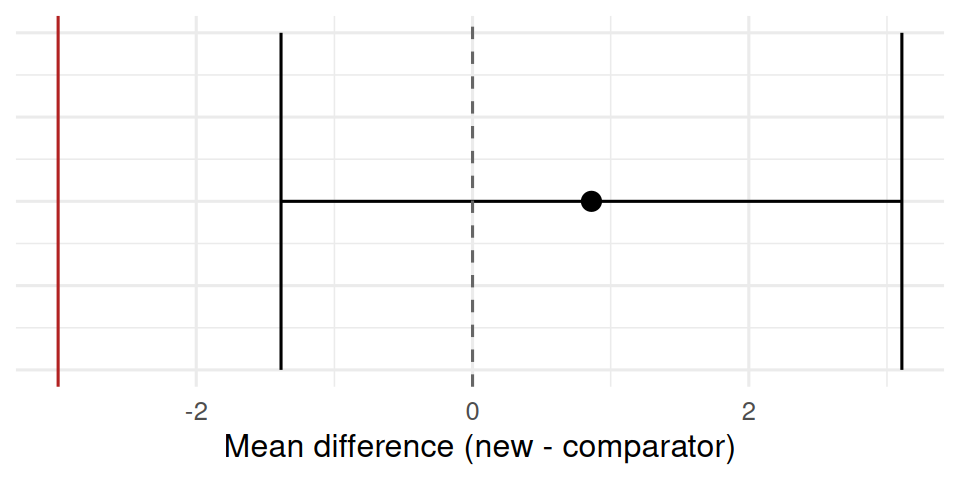
5. Concluding statement
The new treatment had a mean difference of 0.86 versus comparator (95% CI: -1.39 to 3.11). With a pre-specified non-inferiority margin of Δ = 3, the new treatment met the non-inferiority criterion because the lower bound exceeded −Δ.
A word on adaptive designs
Adaptive designs work when the adaptation rules and the alpha spent at each look are pre-specified. Running an interim analysis with the hope of extending the trial if it looks promising — without a pre- specified rule — inflates Type I error and destroys the trial’s inferential warranty.
A common exam trap is to confuse “fails to reject superiority” with “establishes non-inferiority”. They are not the same thing.
Common pitfalls
- Picking the NI margin after seeing the data.
- Using a two-sided superiority test and claiming non-inferiority.
- Running an “interim look” without a pre-specified spending rule.
- Treating equivalence and non-inferiority as interchangeable.
Further reading
- Piaggio G et al. (2012), CONSORT extension for non-inferiority and equivalence trials.
- Jennison C, Turnbull BW. Group Sequential Methods with Applications to Clinical Trials.
- FDA (2016), Non-Inferiority Clinical Trials to Establish Effectiveness.
Session info
sessionInfo()R version 4.5.2 (2025-10-31 ucrt)
Platform: x86_64-w64-mingw32/x64
Running under: Windows 11 x64 (build 26200)
Matrix products: default
LAPACK version 3.12.1
locale:
[1] LC_COLLATE=English_Germany.utf8 LC_CTYPE=English_Germany.utf8
[3] LC_MONETARY=English_Germany.utf8 LC_NUMERIC=C
[5] LC_TIME=English_Germany.utf8
time zone: Europe/Berlin
tzcode source: internal
attached base packages:
[1] stats graphics grDevices utils datasets methods base
other attached packages:
[1] lubridate_1.9.5 forcats_1.0.1 stringr_1.6.0 dplyr_1.2.1
[5] purrr_1.2.2 readr_2.2.0 tidyr_1.3.2 tibble_3.3.1
[9] ggplot2_4.0.3 tidyverse_2.0.0
loaded via a namespace (and not attached):
[1] gtable_0.3.6 jsonlite_2.0.0 compiler_4.5.2 tidyselect_1.2.1
[5] scales_1.4.0 yaml_2.3.12 fastmap_1.2.0 R6_2.6.1
[9] labeling_0.4.3 generics_0.1.4 knitr_1.51 htmlwidgets_1.6.4
[13] pillar_1.11.1 RColorBrewer_1.1-3 tzdb_0.5.0 rlang_1.2.0
[17] stringi_1.8.7 xfun_0.57 S7_0.2.2 otel_0.2.0
[21] timechange_0.4.0 cli_3.6.6 withr_3.0.2 magrittr_2.0.4
[25] digest_0.6.39 grid_4.5.2 hms_1.1.4 lifecycle_1.0.5
[29] vctrs_0.7.3 evaluate_1.0.5 glue_1.8.1 farver_2.1.2
[33] rmarkdown_2.31 tools_4.5.2 pkgconfig_2.0.3 htmltools_0.5.9