library(tidyverse)
library(broom)
set.seed(42)
theme_set(theme_minimal(base_size = 12))Week 3, Session 2 — ANCOVA in RCTs (baseline adjustment)
Course 2 — #courses
Note
Inference labs use the five-step template: Hypothesis → Visualise → Assumptions → Conduct → Conclude.
Learning objectives
- Choose between change scores, post-only, and ANCOVA in an RCT analysis plan.
- Fit an ANCOVA model and read the treatment effect as an adjusted-mean difference.
- Show that ANCOVA is more efficient than the change-score approach when baseline and follow-up are correlated.
Prerequisites
Week 1 regression; Week 2 one-way ANOVA.
Background
In a randomised trial with a continuous outcome measured at baseline and follow-up, three analyses are common: compare the post-intervention means, compare the change scores, or use analysis of covariance (ANCOVA) with baseline as a covariate. Randomisation ensures all three are unbiased in expectation, but they are not equally efficient.
ANCOVA weights the baseline by its observed correlation with the follow-up and is therefore always at least as efficient as the change-score approach, and much more efficient when that correlation is moderate. Change scores are equivalent to ANCOVA with the baseline slope constrained to 1; post-only is ANCOVA with the slope constrained to 0. When neither constraint matches the data, efficiency is lost.
Regression to the mean (Week 4 Session 1) is the mechanical reason ANCOVA wins. Patients with unusually high baselines tend to have lower follow-ups whether they are treated or not; ANCOVA uses that pattern, change-score analysis pretends it does not exist.
Setup
1. Hypothesis
Simulate a trial with baseline and follow-up correlated at r = 0.6, then compare the three analyses.
2. Visualise
n <- 200
baseline <- rnorm(n, 140, 15)
arm <- rep(c("placebo", "active"), each = n / 2)
# true treatment effect on follow-up: -5
followup <- 0.6 * (baseline - 140) + 140 +
  ifelse(arm == "active", -5, 0) + rnorm(n, 0, 12)
dat <- tibble(baseline, followup, arm,
              change = followup - baseline) |>
  mutate(arm = factor(arm, levels = c("placebo", "active")))

ggplot(dat, aes(baseline, followup, colour = arm)) +
  geom_point(alpha = 0.6) +
  geom_smooth(method = "lm", se = FALSE) +
  labs(x = "Baseline", y = "Follow-up")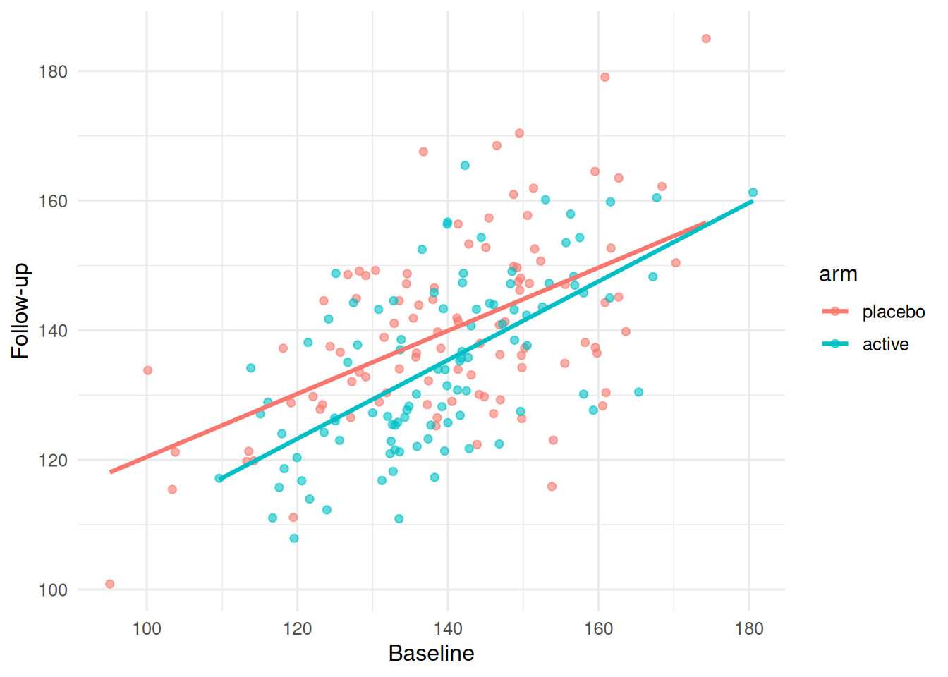
3. Assumptions
Randomisation; linear relationship between baseline and follow-up; equal slopes across arms (tested with an interaction term).
fit_int <- lm(followup ~ arm * baseline, data = dat)
tidy(fit_int) |> filter(term == "armactive:baseline")
# A tibble: 1 × 5
term estimate std.error statistic p.value
<chr> <dbl> <dbl> <dbl> <dbl>
1 armactive:baseline 0.120 0.112 1.07 0.285If the interaction is small, pool the slopes in the ANCOVA.
4. Conduct
fit_post   <- lm(followup ~ arm, data = dat)
fit_change <- lm(change ~ arm, data = dat)
fit_ancova <- lm(followup ~ arm + baseline, data = dat)

bind_rows(
  tidy(fit_post, conf.int = TRUE) |> mutate(model = "post only"),
  tidy(fit_change, conf.int = TRUE) |> mutate(model = "change"),
  tidy(fit_ancova, conf.int = TRUE) |> mutate(model = "ANCOVA")
) |>
  filter(term == "armactive") |>
  dplyr::select(model, estimate, std.error, conf.low, conf.high)
# A tibble: 3 × 5
model estimate std.error conf.low conf.high
<chr> <dbl> <dbl> <dbl> <dbl>
1 post only -5.56 1.95 -9.41 -1.71
2 change -3.76 1.87 -7.44 -0.0760
3 ANCOVA -4.59 1.61 -7.77 -1.41 The three estimates should all be around −5; the ANCOVA standard error should be the smallest.
5. Concluding statement
In a simulated trial (n = 200), ANCOVA estimated the treatment effect at -4.59 units (95% CI -7.77 to -1.41) with a smaller standard error than either the post-only or change-score analyses. ANCOVA is the prespecified primary analysis in most continuous-outcome RCTs.
Say out loud: baseline is not a covariate you can be accused of choosing to inflate the effect — it is fixed before randomisation.
Common pitfalls
- Adjusting for post-baseline covariates (not covered here, but a classic trap).
- Using a change score when baseline and follow-up are strongly correlated.
- Dropping observations with missing baselines instead of imputing or prespecifying a policy.
Further reading
- Senn S (2006), Change from baseline and analysis of covariance…
- Vickers AJ, Altman DG (2001), Analysing controlled trials with…
- ICH E9 (R1) Addendum on Estimands.
Session info
sessionInfo()R version 4.5.2 (2025-10-31 ucrt)
Platform: x86_64-w64-mingw32/x64
Running under: Windows 11 x64 (build 26200)
Matrix products: default
LAPACK version 3.12.1
locale:
[1] LC_COLLATE=English_Germany.utf8 LC_CTYPE=English_Germany.utf8
[3] LC_MONETARY=English_Germany.utf8 LC_NUMERIC=C
[5] LC_TIME=English_Germany.utf8
time zone: Europe/Berlin
tzcode source: internal
attached base packages:
[1] stats graphics grDevices utils datasets methods base
other attached packages:
[1] broom_1.0.12 lubridate_1.9.5 forcats_1.0.1 stringr_1.6.0
[5] dplyr_1.2.1 purrr_1.2.2 readr_2.2.0 tidyr_1.3.2
[9] tibble_3.3.1 ggplot2_4.0.3 tidyverse_2.0.0
loaded via a namespace (and not attached):
[1] Matrix_1.7-5 gtable_0.3.6 jsonlite_2.0.0 compiler_4.5.2
[5] tidyselect_1.2.1 splines_4.5.2 scales_1.4.0 yaml_2.3.12
[9] fastmap_1.2.0 lattice_0.22-9 R6_2.6.1 labeling_0.4.3
[13] generics_0.1.4 knitr_1.51 backports_1.5.1 htmlwidgets_1.6.4
[17] pillar_1.11.1 RColorBrewer_1.1-3 tzdb_0.5.0 rlang_1.2.0
[21] utf8_1.2.6 stringi_1.8.7 xfun_0.57 S7_0.2.2
[25] otel_0.2.0 timechange_0.4.0 cli_3.6.6 mgcv_1.9-4
[29] withr_3.0.2 magrittr_2.0.4 digest_0.6.39 grid_4.5.2
[33] hms_1.1.4 nlme_3.1-169 lifecycle_1.0.5 vctrs_0.7.3
[37] evaluate_1.0.5 glue_1.8.1 farver_2.1.2 rmarkdown_2.31
[41] tools_4.5.2 pkgconfig_2.0.3 htmltools_0.5.9