library(tidyverse)
set.seed(42)
theme_set(theme_minimal(base_size = 12))Week 1, Session 2 — Randomised controlled trials
Course 3 — #courses
Note
Inference lab using the five-step template: Hypothesis → Visualise → Assumptions → Conduct → Conclude.
Learning objectives
- Contrast parallel-group, crossover, cluster, and factorial RCT designs.
- Simulate a parallel-group RCT with a realistic allocation procedure.
- Interpret intention-to-treat (ITT) and per-protocol (PP) analyses and say why they can differ.
Prerequisites
Course 1 inference; t.test(), lm(), and basic tidyverse.
Background
The randomised controlled trial (RCT) is the reference design for causal inference because randomisation balances both measured and unmeasured confounders in expectation. Parallel-group RCTs assign each participant to one arm for the duration of the study. Crossover trials give each participant every treatment in a randomised order and rely on a washout period. Cluster trials randomise groups (clinics, villages) rather than individuals. Factorial trials vary more than one treatment at once and can answer more than one question per patient.
Every RCT has two analyses that will often disagree. Intention-to- treat analyses everyone in the arm they were randomised to, regardless of what they actually received. Per-protocol analyses only those who received the assigned treatment as planned. ITT is conservative for superiority and preserves the randomisation; PP is informative for efficacy in compliant patients but can be biased. Report both, and say which is primary in the protocol.
Allocation concealment — the process that keeps the next assignment unknown until the patient has been enrolled — is not the same as blinding. You can have one without the other, and you need both for the trial to protect itself from selection bias and differential outcome ascertainment.
Setup
1. Hypothesis
Treatment reduces the outcome (a continuous symptom score) relative to placebo. We will also see what happens when 15% of participants cross over from treatment to placebo after randomisation.
2. Visualise
n <- 200
trial <- tibble(
  id    = seq_len(n),
  arm   = sample(rep(c("placebo", "treatment"), each = n / 2)),
  # 15% of treatment arm never take the drug (will be placebo in reality)
  crossed = if_else(arm == "treatment" & runif(n) < 0.15, TRUE, FALSE),
  received = if_else(crossed, "placebo", arm),
  y = rnorm(n, mean = 50, sd = 8) +
      if_else(received == "treatment", -5, 0)
)

trial |>
  ggplot(aes(arm, y, fill = arm)) +
  geom_boxplot(alpha = 0.6, colour = "grey30") +
  labs(x = NULL, y = "Symptom score") +
  theme(legend.position = "none")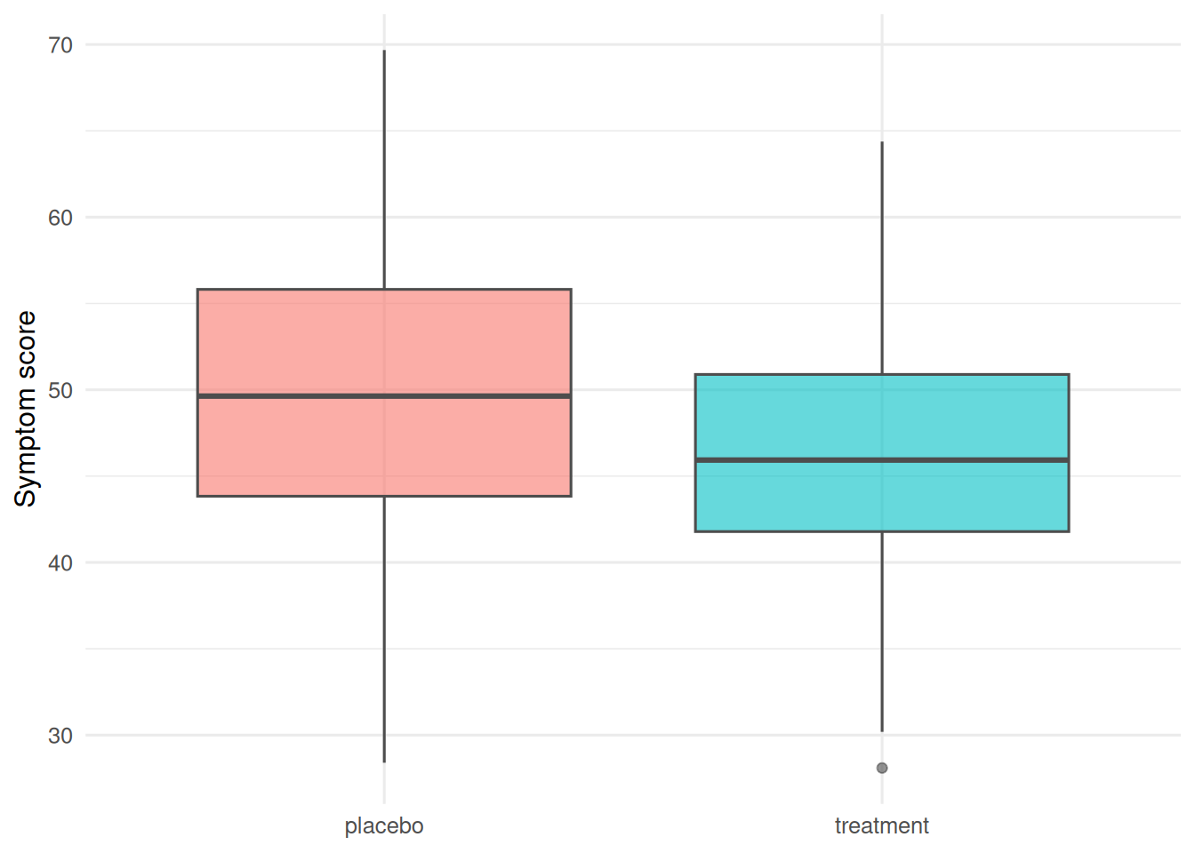
3. Assumptions
A two-sample t-test on the ITT population assumes independent observations within arms and roughly normal residuals within each arm. We do not assume equal variances; t.test() uses Welch by default. The more important assumption is that randomisation worked — that the allocation is independent of every baseline covariate.
trial |>
  group_by(arm) |>
  summarise(mean = mean(y), sd = sd(y), n = n())
# A tibble: 2 × 4
arm mean sd n
<chr> <dbl> <dbl> <int>
1 placebo 49.7 8.14 100
2 treatment 46.1 7.11 1004. Conduct
itt <- with(trial, t.test(y[arm == "treatment"], y[arm == "placebo"]))
pp <- with(subset(trial, !crossed),
           t.test(y[arm == "treatment"], y[arm == "placebo"]))
as_treated <- with(trial,
                   t.test(y[received == "treatment"], y[received == "placebo"]))
itt_diff <- unname(itt$estimate[1] - itt$estimate[2])
pp_diff <- unname(pp$estimate[1] - pp$estimate[2])
at_diff <- unname(as_treated$estimate[1] - as_treated$estimate[2])
itt
    Welch Two Sample t-test

data:  y[arm == "treatment"] and y[arm == "placebo"]
t = -3.3683, df = 194.51, p-value = 0.0009118
alternative hypothesis: true difference in means is not equal to 0
95 percent confidence interval:
 -5.772362 -1.508930
sample estimates:
mean of x mean of y
 46.05756  49.69820
pp
    Welch Two Sample t-test

data:  y[arm == "treatment"] and y[arm == "placebo"]
t = -3.5108, df = 173.65, p-value = 0.0005692
alternative hypothesis: true difference in means is not equal to 0
95 percent confidence interval:
 -6.37476 -1.78660
sample estimates:
mean of x mean of y
 45.61752  49.69820
ITT retains everyone in the randomised arm. The per-protocol subset excludes crossovers; the as-treated comparison groups everyone by treatment received. The latter two generally sacrifice the protection of randomisation. In this simulation crossover is independent of prognosis, so it does not demonstrate bias from informative non-adherence.
5. Concluding statement
In the simulated RCT (n = 200), the treatment-minus-placebo symptom difference was -3.6 under ITT (95% CI: -5.8 to -1.5). The per-protocol difference was -4.1 and the as-treated difference was -3.7. Negative differences favour treatment. These estimates target different comparisons; their ordering can vary.
The practical takeaway is that ITT protects the randomisation, PP answers a different question, and reporting only the one that looks good is a quiet form of bias.
Common pitfalls
- Calling a non-random allocation “randomised” because a coin was flipped after enrolment.
- Reporting only PP and calling it primary.
- Ignoring stratification variables in the analysis when they were used at randomisation.
- Cluster trials analysed as if individuals were independent.
Further reading
- Schulz KF, Altman DG, Moher D (2010), CONSORT 2010 Statement.
- Pocock SJ. Clinical Trials: A Practical Approach.
- Hernán MA, Hernández-Díaz S (2012), Beyond the intention-to-treat in comparative effectiveness research.
Session info
sessionInfo()R version 4.6.1 (2026-06-24)
Platform: x86_64-pc-linux-gnu
Running under: Ubuntu 26.04.1 LTS
Matrix products: default
BLAS: /usr/lib/x86_64-linux-gnu/openblas-pthread/libblas.so.3
LAPACK: /usr/lib/x86_64-linux-gnu/openblas-pthread/libopenblasp-r0.3.32.so; LAPACK version 3.12.0
locale:
[1] LC_CTYPE=C.UTF-8 LC_NUMERIC=C LC_TIME=C.UTF-8
[4] LC_COLLATE=C.UTF-8 LC_MONETARY=C.UTF-8 LC_MESSAGES=C.UTF-8
[7] LC_PAPER=C.UTF-8 LC_NAME=C LC_ADDRESS=C
[10] LC_TELEPHONE=C LC_MEASUREMENT=C.UTF-8 LC_IDENTIFICATION=C
time zone: UTC
tzcode source: system (glibc)
attached base packages:
[1] stats graphics grDevices datasets utils methods base
other attached packages:
[1] lubridate_1.9.5 forcats_1.0.1 stringr_1.6.0 dplyr_1.2.1
[5] purrr_1.2.2 readr_2.2.0 tidyr_1.3.2 tibble_3.3.1
[9] ggplot2_4.0.3 tidyverse_2.0.0
loaded via a namespace (and not attached):
[1] gtable_0.3.6 jsonlite_2.0.0 compiler_4.6.1 renv_1.3.1
[5] tidyselect_1.2.1 scales_1.4.0 yaml_2.3.12 fastmap_1.2.0
[9] R6_2.6.1 labeling_0.4.3 generics_0.1.4 knitr_1.52
[13] htmlwidgets_1.6.4 tzdb_0.5.0 pillar_1.11.1 RColorBrewer_1.1-3
[17] rlang_1.3.0 utf8_1.2.6 stringi_1.8.9 xfun_0.62
[21] S7_0.2.2 otel_0.2.0 timechange_0.4.0 cli_3.6.6
[25] withr_3.0.3 magrittr_2.0.5 digest_0.6.39 grid_4.6.1
[29] hms_1.1.4 lifecycle_1.0.5 vctrs_0.7.3 evaluate_1.0.5
[33] glue_1.8.1 farver_2.1.2 rmarkdown_2.32 tools_4.6.1
[37] pkgconfig_2.0.3 htmltools_0.5.9