library(tidyverse)
set.seed(42)
theme_set(theme_minimal(base_size = 12))Week 1, Session 4 — Bench and translational design
Course 3 — #courses
Note
Inference lab using the five-step template: Hypothesis → Visualise → Assumptions → Conduct → Conclude.
Learning objectives
- Recognise blocking, factorial, and split-plot designs in a bench setting.
- Simulate a 2 × 2 factorial experiment and test the interaction.
- Spot and correct a pseudoreplication error in a cell-culture example.
Prerequisites
Course 2 linear regression and ANOVA; familiarity with the formula interface.
Background
Bench and translational biology lives on small, carefully structured experiments whose designs are often misread as simple one-way comparisons. Blocking groups observations that share a nuisance variable (a batch, a day, a plate) so that comparisons are made within blocks. Factorial designs manipulate two or more factors at once and estimate main effects and interactions from a single experiment. Split-plot designs randomise two factors at different scales — a hard-to-change factor (oven temperature) at the whole- plot level, an easier one (position on the tray) at the sub-plot level — and the analysis must respect that structure.
Pseudoreplication is what happens when the experimental unit and the observational unit are confused. If one animal’s blood is pipetted into ten wells, the ten wells are not ten independent samples; they are ten technical replicates of one biological replicate. Analysing them as independent inflates the apparent sample size, shrinks the standard error, and produces spuriously small p-values. The fix is to aggregate within the experimental unit or use a mixed model that knows about the nested structure.
A useful question to ask before every analysis: what is the unit I could have independently randomised? That is the unit of analysis. If an intervention was applied to a cage but measurements were taken on each mouse, the cage is the unit.
Setup
1. Hypothesis
A drug and a diet each affect a continuous biomarker, and their combination may have a non-additive effect (interaction).
2. Visualise
n_per_cell <- 10
fact <- expand_grid(
  drug = c("no", "yes"),
  diet = c("standard", "modified"),
  rep  = seq_len(n_per_cell)
) |>
  mutate(
    y = 10 +
      (drug == "yes")  * 1.5 +
      (diet == "modified") * 1.0 +
      (drug == "yes" & diet == "modified") * 2.0 +
      rnorm(n(), 0, 1.5)
  )

fact |>
  ggplot(aes(diet, y, fill = drug)) +
  geom_boxplot(alpha = 0.6, colour = "grey30") +
  labs(x = NULL, y = "Biomarker", fill = "Drug")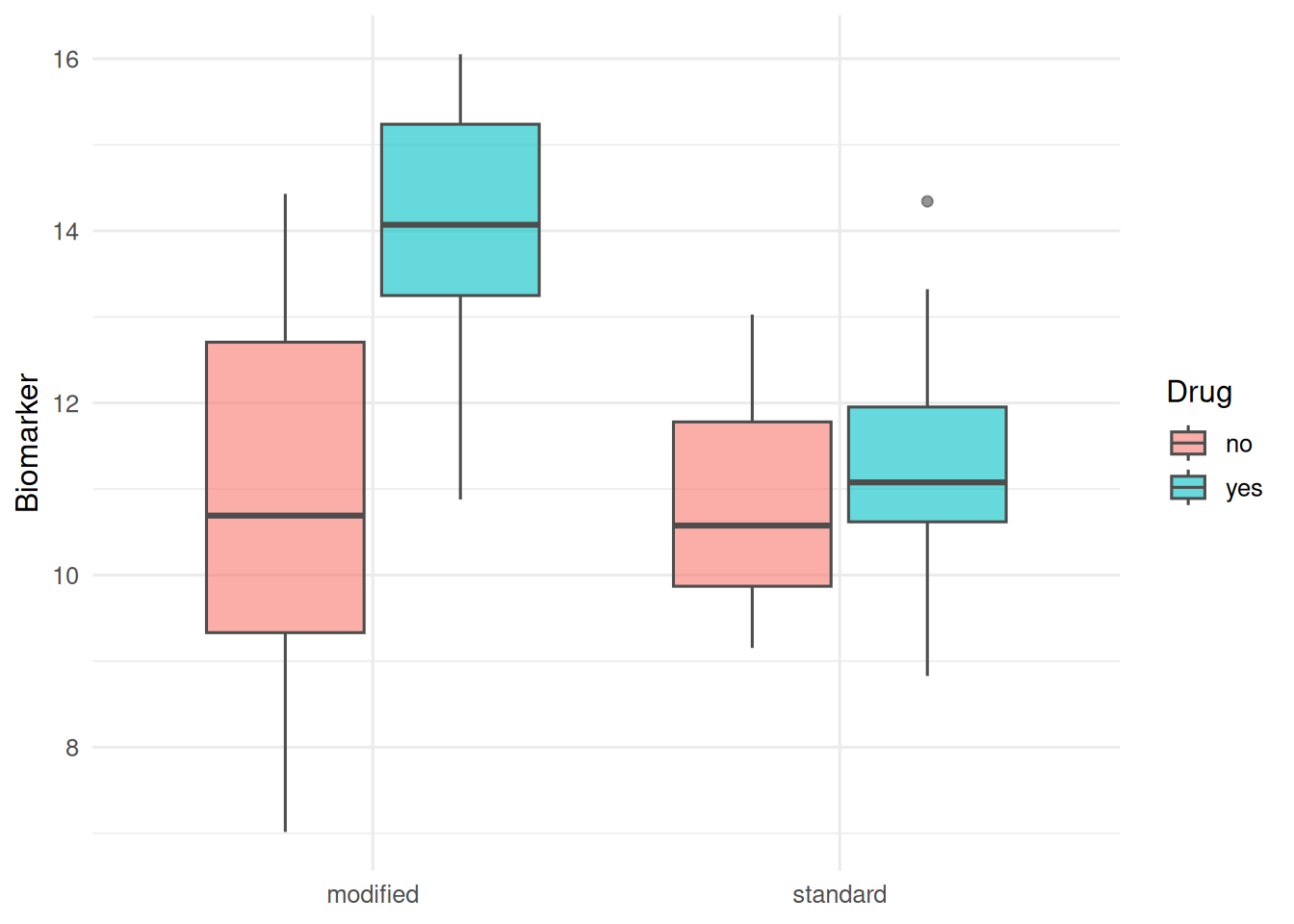
3. Assumptions
Independent observations within each cell (every replicate is a separate biological unit), approximately normal residuals, and equal variance across cells. For the pseudoreplication demonstration we deliberately break the independence assumption.
fact |>
  group_by(drug, diet) |>
  summarise(mean = mean(y), sd = sd(y), n = n(), .groups = "drop")
# A tibble: 4 × 5
drug diet mean sd n
<chr> <chr> <dbl> <dbl> <int>
1 no modified 10.8 2.45 10
2 no standard 10.8 1.25 10
3 yes modified 14.0 1.67 10
4 yes standard 11.2 1.73 104. Conduct
fit <- lm(y ~ drug * diet, data = fact)
anova(fit)
Analysis of Variance Table
Response: y
Df Sum Sq Mean Sq F value Pr(>F)
drug 1 32.603 32.603 9.7626 0.00351 **
diet 1 17.624 17.624 5.2774 0.02753 *
drug:diet 1 19.424 19.424 5.8162 0.02110 *
Residuals 36 120.226 3.340
---
Signif. codes: 0 '***' 0.001 '**' 0.01 '*' 0.05 '.' 0.1 ' ' 1Now a pseudoreplication error. Suppose each biological replicate was measured three times (technical replicates) and we naively treated the 3 × rows as independent.
pseudo <- fact |>
  slice(rep(seq_len(n()), each = 3)) |>
  mutate(tech_noise = rnorm(n(), 0, 0.3),
         y = y + tech_noise)

fit_bad  <- lm(y ~ drug * diet, data = pseudo)
fit_good <- lm(y ~ drug * diet, data = fact)  # aggregated (original)

bind_rows(
  bad  = broom::tidy(fit_bad)  |> filter(term == "drugyes:dietmodified"),
  good = broom::tidy(fit_good) |> filter(term == "drugyes:dietmodified"),
  .id = "analysis"
)
# A tibble: 0 × 6
# ℹ 6 variables: analysis <chr>, term <chr>, estimate <dbl>, std.error <dbl>,
# statistic <dbl>, p.value <dbl>The point estimate barely moves; the standard error in the bad analysis is smaller because the apparent n is three times larger.
5. Concluding statement
In a simulated 2 × 2 factorial experiment (10 biological replicates per cell), there was evidence of an interaction between drug and diet on the biomarker (F and p from the ANOVA table above). Naive analysis of technical replicates as independent observations shrinks the standard error of the interaction estimate without changing the point estimate — a textbook pseudoreplication artefact.
A slide that shows the same point estimate with two CIs, one wide and one narrow, is usually the clearest way to convey pseudoreplication to a wet-lab audience.
Common pitfalls
- Counting wells, sections, or reads as independent samples.
- Forgetting to include the block in the model when the design was blocked.
- Running a one-way ANOVA on a factorial design and losing the interaction.
- Split-plot designs analysed with a single-error-term model.
Further reading
- Montgomery DC. Design and Analysis of Experiments.
- Lazic SE (2010), The problem of pseudoreplication in neuroscientific studies.
- Festing MFW (2006), Design and statistical methods in studies using animal models.
Session info
sessionInfo()R version 4.5.2 (2025-10-31 ucrt)
Platform: x86_64-w64-mingw32/x64
Running under: Windows 11 x64 (build 26200)
Matrix products: default
LAPACK version 3.12.1
locale:
[1] LC_COLLATE=English_Germany.utf8 LC_CTYPE=English_Germany.utf8
[3] LC_MONETARY=English_Germany.utf8 LC_NUMERIC=C
[5] LC_TIME=English_Germany.utf8
time zone: Europe/Berlin
tzcode source: internal
attached base packages:
[1] stats graphics grDevices utils datasets methods base
other attached packages:
[1] lubridate_1.9.5 forcats_1.0.1 stringr_1.6.0 dplyr_1.2.1
[5] purrr_1.2.2 readr_2.2.0 tidyr_1.3.2 tibble_3.3.1
[9] ggplot2_4.0.3 tidyverse_2.0.0
loaded via a namespace (and not attached):
[1] gtable_0.3.6 jsonlite_2.0.0 compiler_4.5.2 tidyselect_1.2.1
[5] scales_1.4.0 yaml_2.3.12 fastmap_1.2.0 R6_2.6.1
[9] labeling_0.4.3 generics_0.1.4 knitr_1.51 backports_1.5.1
[13] htmlwidgets_1.6.4 pillar_1.11.1 RColorBrewer_1.1-3 tzdb_0.5.0
[17] rlang_1.2.0 utf8_1.2.6 broom_1.0.12 stringi_1.8.7
[21] xfun_0.57 S7_0.2.2 otel_0.2.0 timechange_0.4.0
[25] cli_3.6.6 withr_3.0.2 magrittr_2.0.4 digest_0.6.39
[29] grid_4.5.2 hms_1.1.4 lifecycle_1.0.5 vctrs_0.7.3
[33] evaluate_1.0.5 glue_1.8.1 farver_2.1.2 rmarkdown_2.31
[37] tools_4.5.2 pkgconfig_2.0.3 htmltools_0.5.9