library(tidyverse)
library(lme4)
library(glmmTMB)
library(geepack)
set.seed(42)
theme_set(theme_minimal(base_size = 12))Week 2, Session 4 — GLMMs and GEE
Course 3 — #courses
Note
Inference lab using the five-step template: Hypothesis → Visualise → Assumptions → Conduct → Conclude.
Learning objectives
- Fit a binary GLMM for clustered data with
lme4::glmerand withglmmTMB. - Fit a GEE with
geepack::geeglmand compare coefficient interpretations. - Say why GLMM and GEE estimate different things (subject-specific vs population-average).
Prerequisites
Week 2 Session 3 (linear mixed models) and Course 2 logistic regression.
Background
For binary outcomes in clustered data, the two standard approaches are generalised linear mixed models (GLMM) and generalised estimating equations (GEE). A GLMM is a random-effects model on the link scale; its fixed-effect coefficients are conditional on the random effect and describe subject-specific effects. A GEE fits a marginal model using a working correlation structure; its coefficients describe population-averaged effects. For logistic models, the two will not in general agree even when both are correctly specified.
lme4::glmer is the classic random-effects fitter; glmmTMB handles larger and more complex random structures including correlated random effects and zero-inflated distributions. geepack fits GEEs with several working correlation choices; the standard errors are robust to misspecification of the correlation structure but the point estimate can shift.
The choice between GLMM and GEE is not a statistical technicality; it is a choice of estimand. If you care about what happens inside a person over time, you want a GLMM. If you care about a population- average effect for policy or for a marginal treatment effect, you want a GEE (or a marginalised GLMM).
Setup
1. Hypothesis
Treatment reduces the probability of a repeated binary event in a clustered study (clusters = clinics). The true log-odds fixed effect is −0.5.
2. Visualise
J  <- 30
nj <- 20
dat <- tibble(
  clinic = factor(rep(seq_len(J), each = nj)),
  trt    = rbinom(J * nj, 1, 0.5),
  u      = rep(rnorm(J, 0, 0.8), each = nj)
) |>
  mutate(lp = -0.5 * trt + u,
         y  = rbinom(n(), 1, plogis(lp)))

dat |>
  group_by(clinic, trt) |>
  summarise(p = mean(y), .groups = "drop") |>
  ggplot(aes(factor(trt), p)) +
  geom_boxplot(alpha = 0.6) +
  labs(x = "Treatment", y = "Event probability per clinic")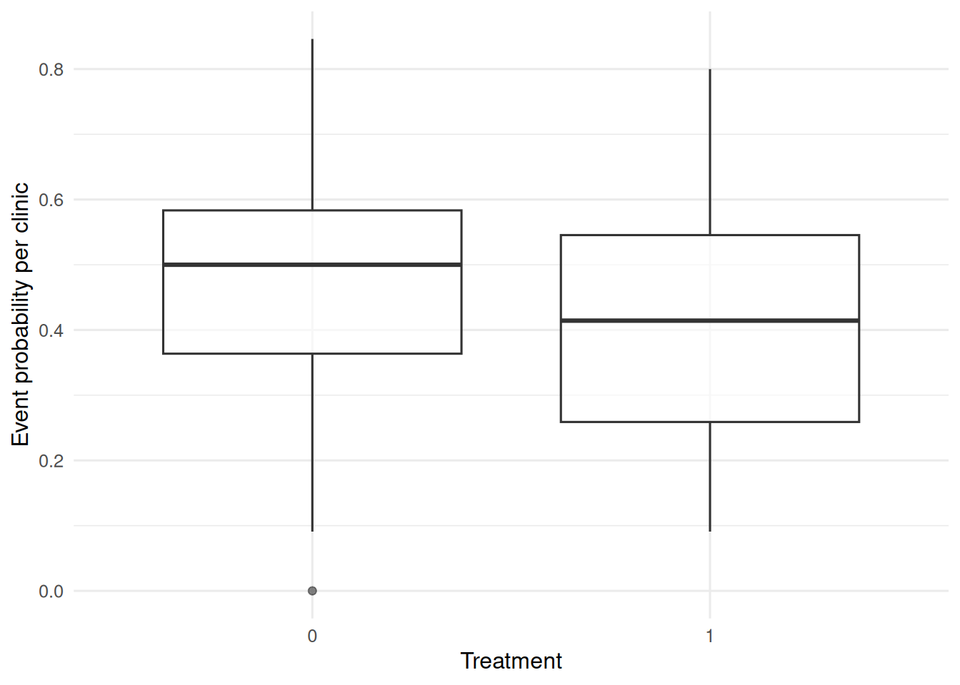
3. Assumptions
GLMM: normal random intercepts for clinic, correct link. GEE: correct mean structure; standard errors robust to working correlation.
4. Conduct
fit_glmer <- glmer(y ~ trt + (1 | clinic),
                   data = dat, family = binomial)
fit_tmb   <- glmmTMB(y ~ trt + (1 | clinic),
                     data = dat, family = binomial)
fit_gee   <- geeglm(y ~ trt, id = clinic, data = dat,
                    family = binomial, corstr = "exchangeable")

summary(fit_glmer)$coefficients
Estimate Std. Error z value Pr(>|z|)
(Intercept) -0.1276856 0.1482618 -0.8612175 0.3891183
trt -0.1813540 0.1716005 -1.0568383 0.2905854summary(fit_tmb)$coefficients$cond Estimate Std. Error z value Pr(>|z|)
(Intercept) -0.1276897 0.1483164 -0.8609276 0.3892779
trt -0.1813538 0.1717070 -1.0561817 0.2908852
attr(,"ddf")
[1] "asymptotic"summary(fit_gee)$coefficients Estimate Std.err Wald Pr(>|W|)
(Intercept) -0.1198702 0.1331773 0.8101448 0.3680774
trt -0.1714235 0.1612817 1.1297196 0.2878352bind_rows(
glmer = broom.mixed::tidy(fit_glmer, effects = "fixed"),
glmmTMB = broom.mixed::tidy(fit_tmb, effects = "fixed"),
gee = broom::tidy(fit_gee),
.id = "model"
) |>
filter(term == "trt") |>
select(model, estimate, std.error)# A tibble: 3 × 3
model estimate std.error
<chr> <dbl> <dbl>
1 glmer -0.181 0.172
2 glmmTMB -0.181 0.172
3 gee -0.171 0.1615. Concluding statement
The GLMM gave a subject-specific treatment log-odds of about -0.18; the GEE gave a population- averaged log-odds of about -0.17. The GEE estimate is typically attenuated toward zero relative to the GLMM; both are correct answers to different questions.
Make sure students report which correlation structure they used in the GEE; it matters for small samples even though the standard errors are robust.
Common pitfalls
- Comparing GLMM and GEE coefficients as if they estimate the same thing.
- Using a working independence structure in GEE when clusters are large and treatment is heterogeneous within them.
- Ignoring overdispersion in a count GLMM by assuming Poisson when negative binomial fits better.
- Fitting a GLMM with too few clusters (< 10) and trusting the variance component.
Further reading
- Liang KY, Zeger SL (1986), Longitudinal data analysis using generalized linear models.
- Zeger SL, Liang KY, Albert PS (1988), Models for longitudinal data: a generalized estimating equation approach.
- Brooks ME et al. (2017), glmmTMB balances speed and flexibility.
Session info
sessionInfo()R version 4.5.2 (2025-10-31 ucrt)
Platform: x86_64-w64-mingw32/x64
Running under: Windows 11 x64 (build 26200)
Matrix products: default
LAPACK version 3.12.1
locale:
[1] LC_COLLATE=English_Germany.utf8 LC_CTYPE=English_Germany.utf8
[3] LC_MONETARY=English_Germany.utf8 LC_NUMERIC=C
[5] LC_TIME=English_Germany.utf8
time zone: Europe/Berlin
tzcode source: internal
attached base packages:
[1] stats graphics grDevices utils datasets methods base
other attached packages:
[1] geepack_1.3.13 glmmTMB_1.1.14 lme4_2.0-1 Matrix_1.7-5
[5] lubridate_1.9.5 forcats_1.0.1 stringr_1.6.0 dplyr_1.2.1
[9] purrr_1.2.2 readr_2.2.0 tidyr_1.3.2 tibble_3.3.1
[13] ggplot2_4.0.3 tidyverse_2.0.0
loaded via a namespace (and not attached):
[1] gtable_0.3.6 TMB_1.9.21 xfun_0.57
[4] htmlwidgets_1.6.4 lattice_0.22-9 tzdb_0.5.0
[7] numDeriv_2016.8-1.1 vctrs_0.7.3 tools_4.5.2
[10] Rdpack_2.6.6 generics_0.1.4 parallel_4.5.2
[13] sandwich_3.1-1 pkgconfig_2.0.3 RColorBrewer_1.1-3
[16] S7_0.2.2 lifecycle_1.0.5 compiler_4.5.2
[19] farver_2.1.2 codetools_0.2-20 htmltools_0.5.9
[22] yaml_2.3.12 furrr_0.4.0 pillar_1.11.1
[25] nloptr_2.2.1 MASS_7.3-65 broom.mixed_0.2.9.7
[28] reformulas_0.4.4 boot_1.3-32 multcomp_1.4-30
[31] parallelly_1.47.0 nlme_3.1-169 tidyselect_1.2.1
[34] digest_0.6.39 future_1.70.0 mvtnorm_1.3-7
[37] stringi_1.8.7 listenv_0.10.1 labeling_0.4.3
[40] splines_4.5.2 fastmap_1.2.0 grid_4.5.2
[43] cli_3.6.6 magrittr_2.0.4 utf8_1.2.6
[46] survival_3.8-6 broom_1.0.12 TH.data_1.1-5
[49] withr_3.0.2 backports_1.5.1 scales_1.4.0
[52] timechange_0.4.0 estimability_1.5.1 rmarkdown_2.31
[55] globals_0.19.1 emmeans_2.0.3 otel_0.2.0
[58] zoo_1.8-15 hms_1.1.4 coda_0.19-4.1
[61] evaluate_1.0.5 knitr_1.51 rbibutils_2.4.1
[64] mgcv_1.9-4 rlang_1.2.0 Rcpp_1.1.1-1.1
[67] xtable_1.8-8 glue_1.8.1 minqa_1.2.8
[70] jsonlite_2.0.0 R6_2.6.1