Week 2, Session 3 — Linear mixed models with lme4

Course 3 — #courses

Author

R. Heller

Note

Inference lab using the five-step template: Hypothesis → Visualise → Assumptions → Conduct → Conclude.

Learning objectives

Fit random-intercept and random-slope linear mixed models to longitudinal data.
Test whether adding a random slope improves fit (likelihood ratio test with ML).
Interpret REML estimates of variance components.

Prerequisites

Course 2 regression; familiarity with lm().

Background

Longitudinal data have two sources of variation: differences between people and differences over time within a person. A random-intercept model lets each person have their own average level; a random-slope model lets each person also have their own rate of change. When the slopes genuinely vary, omitting the random slope underestimates the standard error of the fixed-effect slope and produces p-values that are too small.

REML (restricted maximum likelihood) is the default because it gives unbiased estimates of the variance components by integrating out the fixed effects. It is the right choice for reporting variance components. For comparing models that differ in fixed effects, you must refit with ML (likelihood ratio tests on REML fits are invalid); for comparing models that differ only in random effects, REML is fine.

A common misstep is to interpret the variance of the random intercept as the “within-subject variance”. It is the between- subject variance of the intercept. The within-subject variance is the residual variance, σ², once the random effects are accounted for.

Setup

library(tidyverse)
library(lme4)
library(lmerTest)
set.seed(42)
theme_set(theme_minimal(base_size = 12))

1. Hypothesis

In the sleepstudy data, reaction time increases with days of sleep deprivation, and the rate of increase varies by subject.

2. Visualise

data(sleepstudy, package = "lme4")

sleepstudy |>
  ggplot(aes(Days, Reaction, group = Subject)) +
  geom_line(alpha = 0.3) +
  geom_smooth(aes(group = 1), method = "lm", se = FALSE,
              colour = "firebrick") +
  labs(x = "Days of deprivation", y = "Reaction time (ms)")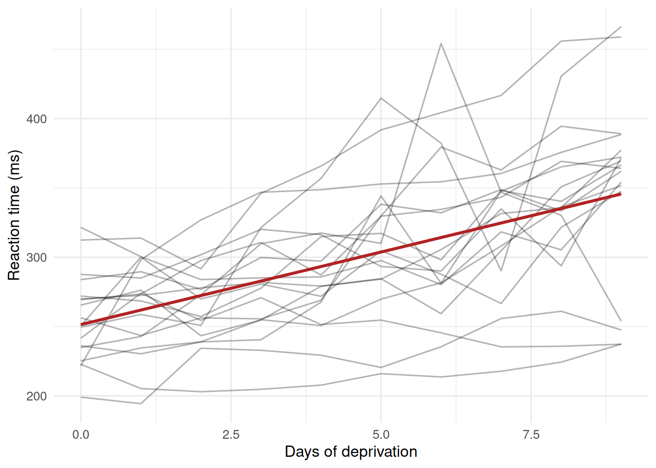

3. Assumptions

Linear relationship between Days and Reaction for each subject; normally distributed random intercepts and slopes (if included); residuals independent within and across subjects after random effects account for clustering; approximately constant residual variance.

4. Conduct

ri <- lmer(Reaction ~ Days + (1 | Subject),
           data = sleepstudy, REML = TRUE)
rs <- lmer(Reaction ~ Days + (Days | Subject),
           data = sleepstudy, REML = TRUE)
summary(rs)

Linear mixed model fit by REML. t-tests use Satterthwaite's method [
lmerModLmerTest]
Formula: Reaction ~ Days + (Days | Subject)
   Data: sleepstudy

REML criterion at convergence: 1743.6

Scaled residuals: 
    Min      1Q  Median      3Q     Max 
-3.9536 -0.4634  0.0231  0.4634  5.1793 

Random effects:
 Groups   Name        Variance Std.Dev. Corr 
 Subject  (Intercept) 612.10   24.741        
          Days         35.07    5.922   0.07 
 Residual             654.94   25.592        
Number of obs: 180, groups:  Subject, 18

Fixed effects:
            Estimate Std. Error      df t value Pr(>|t|)    
(Intercept)  251.405      6.825  17.000  36.838  < 2e-16 ***
Days          10.467      1.546  17.000   6.771 3.26e-06 ***
---
Signif. codes:  0 '***' 0.001 '**' 0.01 '*' 0.05 '.' 0.1 ' ' 1

Correlation of Fixed Effects:
     (Intr)
Days -0.138

# LRT on REML OK here because only random-effects structure differs,
# but we use REFIT = TRUE in anova() to get correct comparison.
anova(ri, rs, refit = FALSE)

Data: sleepstudy
Models:
ri: Reaction ~ Days + (1 | Subject)
rs: Reaction ~ Days + (Days | Subject)
   npar    AIC    BIC  logLik -2*log(L)  Chisq Df Pr(>Chisq)    
ri    4 1794.5 1807.2 -893.23    1786.5                         
rs    6 1755.6 1774.8 -871.81    1743.6 42.837  2   4.99e-10 ***
---
Signif. codes:  0 '***' 0.001 '**' 0.01 '*' 0.05 '.' 0.1 ' ' 1

# Fit with ML if the fixed effects changed
fm_ml <- lmer(Reaction ~ Days + (Days | Subject),
              data = sleepstudy, REML = FALSE)
fm_ml

Linear mixed model fit by maximum likelihood  ['lmerModLmerTest']
Formula: Reaction ~ Days + (Days | Subject)
   Data: sleepstudy
      AIC       BIC    logLik -2*log(L)  df.resid 
1763.9393 1783.0971 -875.9697 1751.9393       174 
Random effects:
 Groups   Name        Std.Dev. Corr 
 Subject  (Intercept) 23.780        
          Days         5.717   0.08 
 Residual             25.592        
Number of obs: 180, groups:  Subject, 18
Fixed Effects:
(Intercept)         Days  
     251.41        10.47

sleepstudy |>
  mutate(fit_rs = predict(rs)) |>
  ggplot(aes(Days, Reaction, group = Subject)) +
  geom_point(alpha = 0.4) +
  geom_line(aes(y = fit_rs), colour = "steelblue") +
  facet_wrap(~ Subject, ncol = 6) +
  theme(strip.text = element_text(size = 7))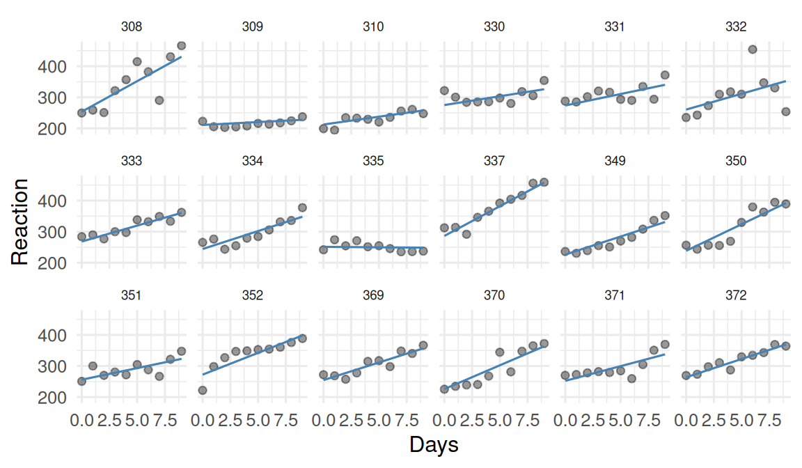

5. Concluding statement

In the sleepstudy data, reaction time increased by about 10.5 ms per day of deprivation, with substantial subject-to-subject variation in slope (SD ≈ 5.9 ms/day). Adding a random slope significantly improved fit over a random-intercept model (likelihood-ratio test p < 0.001).

Emphasise that significance testing for random effects is at the boundary of the parameter space, so the reference distribution is a mixture of chi-squares. lmerTest and anova() do this for you.

Common pitfalls

Testing random-effects with REML-based LRTs without refitting.
Ignoring the random slope when slopes clearly vary.
Treating the Intercept variance as the within-subject error.
Using p-values from the Wald z on small samples.

Session info

sessionInfo()

R version 4.4.1 (2024-06-14)
Platform: x86_64-pc-linux-gnu
Running under: Ubuntu 24.04.4 LTS

Matrix products: default
BLAS:   /usr/lib/x86_64-linux-gnu/openblas-pthread/libblas.so.3 
LAPACK: /usr/lib/x86_64-linux-gnu/openblas-pthread/libopenblasp-r0.3.26.so;  LAPACK version 3.12.0

locale:
 [1] LC_CTYPE=C.UTF-8       LC_NUMERIC=C           LC_TIME=C.UTF-8       
 [4] LC_COLLATE=C.UTF-8     LC_MONETARY=C.UTF-8    LC_MESSAGES=C.UTF-8   
 [7] LC_PAPER=C.UTF-8       LC_NAME=C              LC_ADDRESS=C          
[10] LC_TELEPHONE=C         LC_MEASUREMENT=C.UTF-8 LC_IDENTIFICATION=C   

time zone: UTC
tzcode source: system (glibc)

attached base packages:
[1] stats     graphics  grDevices utils     datasets  methods   base     

other attached packages:
 [1] lmerTest_3.2-1  lme4_2.0-1      Matrix_1.7-0    lubridate_1.9.5
 [5] forcats_1.0.1   stringr_1.6.0   dplyr_1.2.1     purrr_1.2.2    
 [9] readr_2.2.0     tidyr_1.3.2     tibble_3.3.1    ggplot2_4.0.3  
[13] tidyverse_2.0.0

loaded via a namespace (and not attached):
 [1] generics_0.1.4      stringi_1.8.7       lattice_0.22-6     
 [4] hms_1.1.4           digest_0.6.39       magrittr_2.0.5     
 [7] evaluate_1.0.5      grid_4.4.1          timechange_0.4.0   
[10] RColorBrewer_1.1-3  fastmap_1.2.0       jsonlite_2.0.0     
[13] mgcv_1.9-1          scales_1.4.0        numDeriv_2016.8-1.1
[16] reformulas_0.4.4    Rdpack_2.6.6        cli_3.6.6          
[19] rlang_1.2.0         rbibutils_2.4.1     splines_4.4.1      
[22] withr_3.0.2         yaml_2.3.12         otel_0.2.0         
[25] tools_4.4.1         tzdb_0.5.0          nloptr_2.2.1       
[28] minqa_1.2.8         boot_1.3-30         vctrs_0.7.3        
[31] R6_2.6.1            lifecycle_1.0.5     htmlwidgets_1.6.4  
[34] MASS_7.3-60.2       pkgconfig_2.0.3     pillar_1.11.1      
[37] gtable_0.3.6        glue_1.8.1          Rcpp_1.1.1-1.1     
[40] xfun_0.57           tidyselect_1.2.1    knitr_1.51         
[43] farver_2.1.2        htmltools_0.5.9     nlme_3.1-164       
[46] labeling_0.4.3      rmarkdown_2.31      compiler_4.4.1     
[49] S7_0.2.2

Learning objectives

Prerequisites

Background

Setup

1. Hypothesis

2. Visualise

3. Assumptions

4. Conduct

5. Concluding statement

Common pitfalls

Further reading

Session info

Related labs