library(tidyverse)
library(forecast)
library(changepoint)
set.seed(42)
theme_set(theme_minimal(base_size = 12))Week 2, Session 5 — Time series basics
Course 3 — #courses
Note
Inference lab using the five-step template: Hypothesis → Visualise → Assumptions → Conduct → Conclude.
Learning objectives
- Decompose a seasonal time series into trend, seasonal, and residual components.
- Fit an ARIMA model automatically with
forecast::auto.arima. - Detect a mean shift using
changepoint::cpt.mean.
Prerequisites
Course 2 regression; basic familiarity with the ts class.
Background
A time series differs from cross-sectional data in one crucial way: observations close in time are correlated with one another, so standard errors based on independence are wrong. Classical decomposition splits a series into a slowly varying trend, a periodic seasonal component, and a residual. ARIMA models capture the residual autocorrelation with autoregressive and moving-average terms, possibly after differencing to remove a unit root.
Change-point detection asks a different question: given a series, when (if ever) did the underlying mean or variance shift? The changepoint package implements several methods; cpt.mean with a penalised likelihood criterion is a common starting point. In epidemiology, change-points flag outbreaks, policy changes, and data-collection transitions.
A seasonally adjusted series is not the same as a detrended series. Seasonal adjustment removes only the regular period; detrending removes the slow evolution. Most anomalies you care about (an outbreak, an intervention) live in what remains.
Setup
1. Hypothesis
A simulated monthly series has a linear trend, a yearly seasonal cycle, and a mean shift at month 80. Decomposition, ARIMA, and change-point detection should each recover an interpretable piece.
2. Visualise
months <- 144
t  <- seq_len(months)
trend <- 0.08 * t
season <- 4 * sin(2 * pi * t / 12)
shift  <- if_else(t >= 80, 5, 0)
y      <- 20 + trend + season + shift + rnorm(months, 0, 1.5)
ts_y   <- ts(y, frequency = 12, start = c(2014, 1))

autoplot(ts_y) +
  labs(x = "Year", y = "Simulated rate")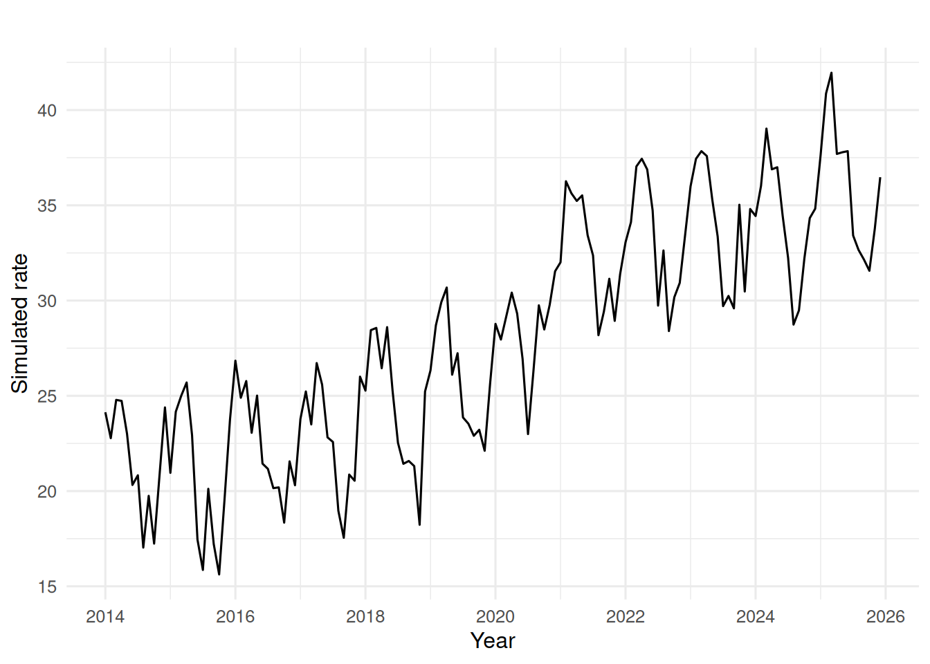
3. Assumptions
STL decomposition assumes the seasonal period is fixed and known. ARIMA assumes a linear, time-invariant generating process after differencing. cpt.mean assumes the variance is approximately constant — change-points in variance would need cpt.var.
4. Conduct
decomp <- stl(ts_y, s.window = "periodic")
autoplot(decomp)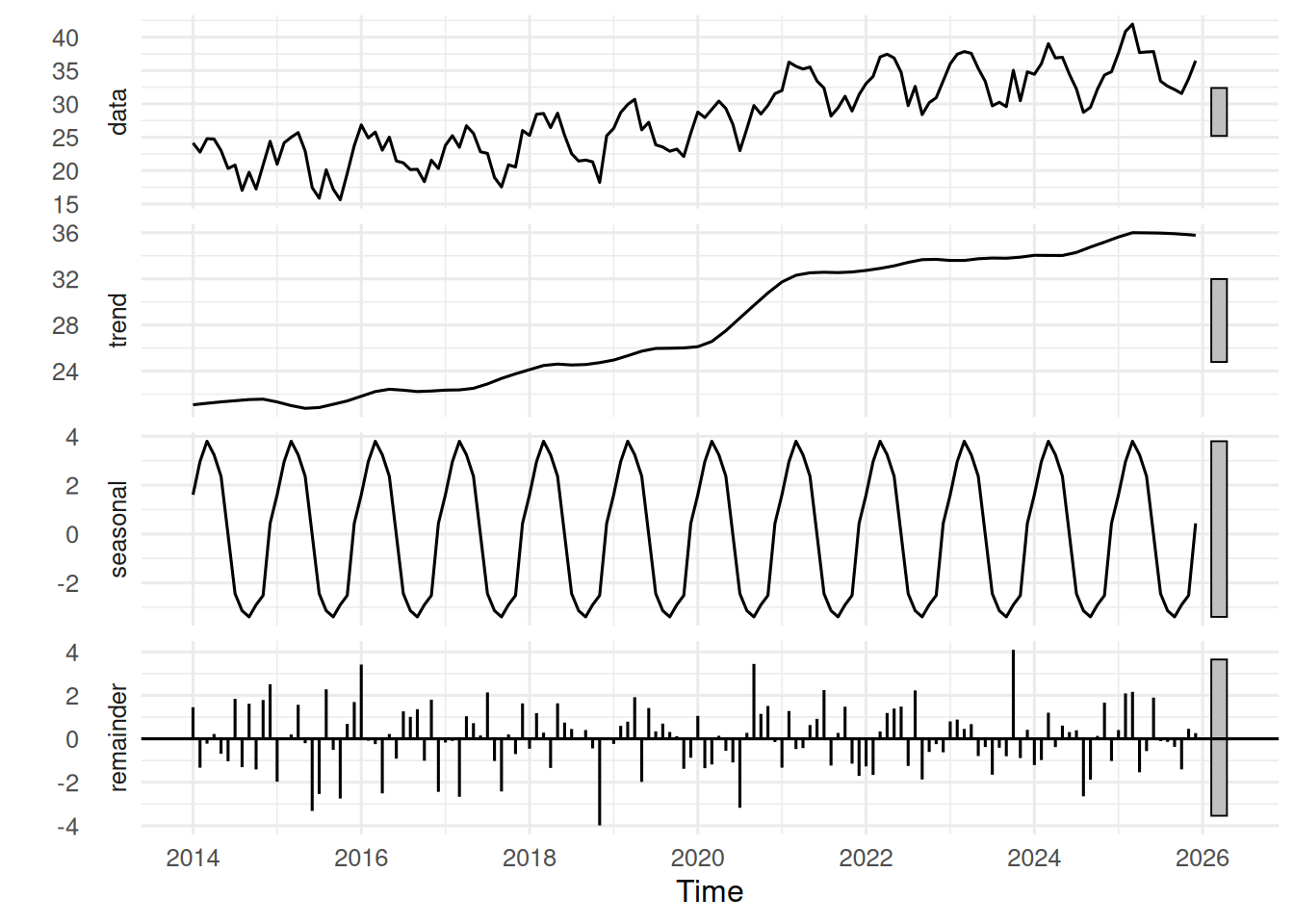
fit_arima <- auto.arima(ts_y)
fit_arima
Series: ts_y
ARIMA(3,0,0)(0,1,1)[12] with drift
Coefficients:
ar1 ar2 ar3 sma1 drift
0.2914 0.2103 0.1666 -0.8570 0.1238
s.e. 0.0862 0.0889 0.0874 0.1125 0.0114
sigma^2 = 3.51: log likelihood = -275.6
AIC=563.2 AICc=563.87 BIC=580.49fc <- forecast(fit_arima, h = 12)
autoplot(fc) +
labs(x = "Year", y = "Simulated rate")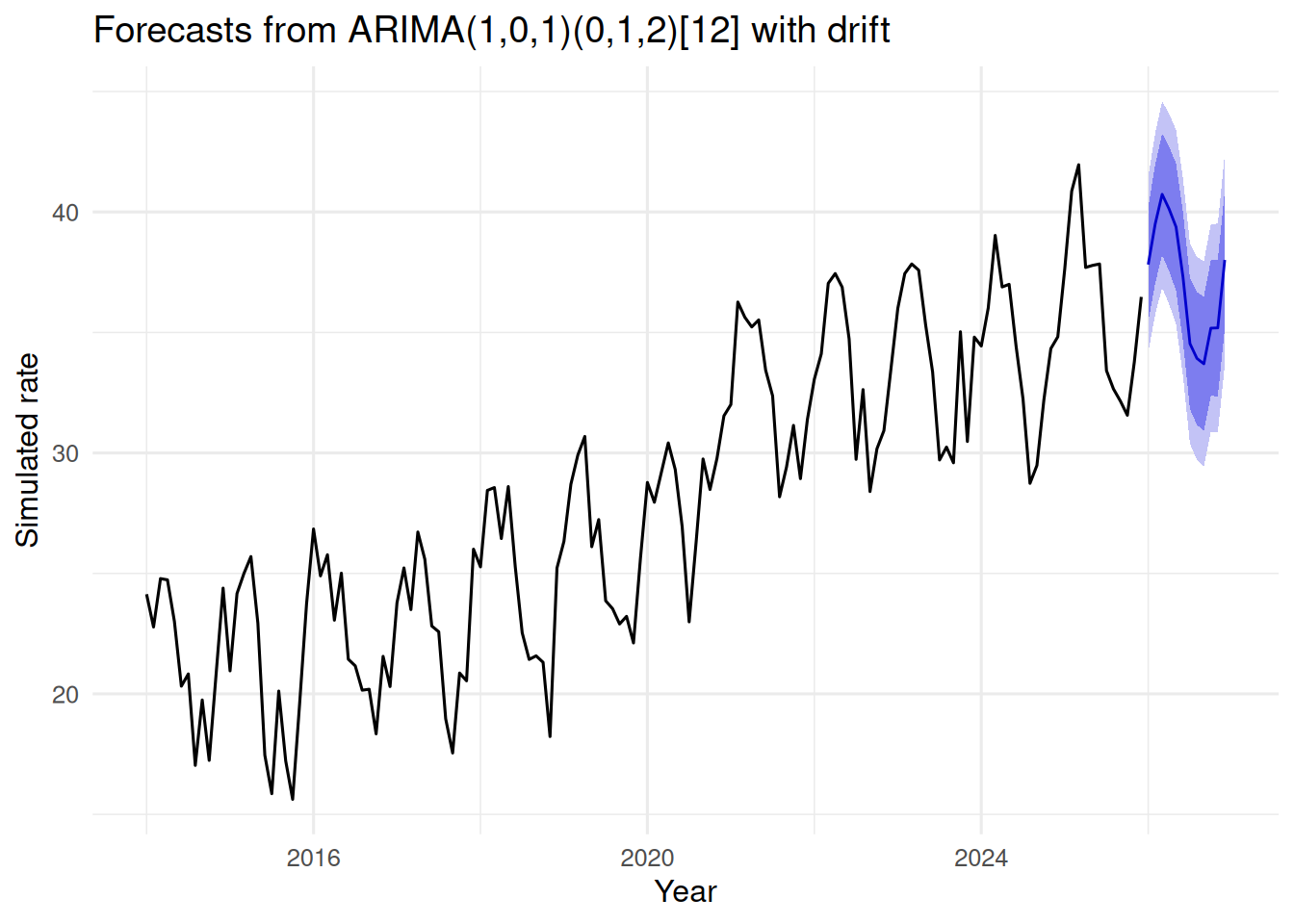
cpt <- cpt.mean(as.numeric(ts_y), method = "PELT")
cpts(cpt)
[1] 5 11 17 23 29 36 43 47 54 59 66 72 77 80 85 90 97 102 108
[20] 113 119 126 130 132 138tibble(t = t, y = as.numeric(ts_y)) |>
ggplot(aes(t, y)) +
geom_line() +
geom_vline(xintercept = cpts(cpt), linetype = "dashed",
colour = "firebrick") +
labs(x = "Month index", y = "Rate")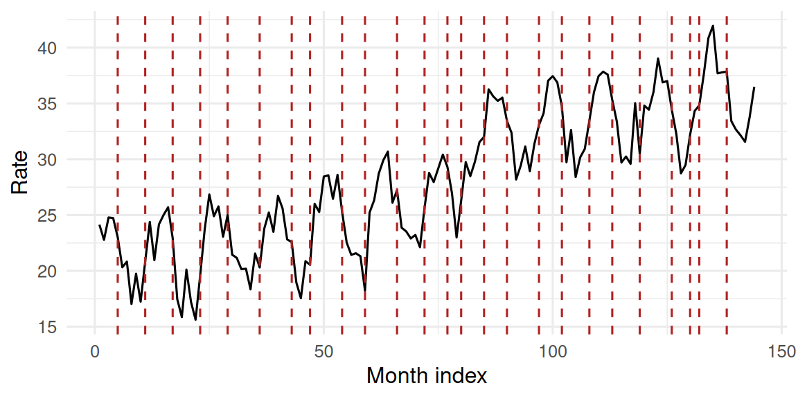
5. Concluding statement
STL cleanly separated a linear trend, a 12-month seasonal cycle, and a residual containing the simulated mean shift.
auto.arimaselected 3, 0, 0, 1, 12, 0, 1 (p, q, P, Q, frequency, d, D). PELT detected change-points at months 5, 11, 17, 23, 29, 36, 43, 47, 54, 59, 66, 72, 77, 80, 85, 90, 97, 102, 108, 113, 119, 126, 130, 132, 138, close to the simulated truth of 80.
When students see ARIMA output, reinforce that AIC is comparing candidates on the same series — the absolute number has no interpretation.
Common pitfalls
- Using daily ARIMA on weekly-seasonal data without telling the model the period.
- Calling every bump a change-point; penalise harder and re-run.
- Using
lm()on a time series as if residuals were independent. - Forecasting far beyond the observed period without widening the intervals in the report.
Further reading
- Hyndman RJ, Athanasopoulos G. Forecasting: Principles and Practice.
- Killick R, Fearnhead P, Eckley IA (2012), Optimal detection of changepoints with a linear computational cost.
- Box GEP, Jenkins GM. Time Series Analysis: Forecasting and Control.
Session info
sessionInfo()R version 4.5.2 (2025-10-31 ucrt)
Platform: x86_64-w64-mingw32/x64
Running under: Windows 11 x64 (build 26200)
Matrix products: default
LAPACK version 3.12.1
locale:
[1] LC_COLLATE=English_Germany.utf8 LC_CTYPE=English_Germany.utf8
[3] LC_MONETARY=English_Germany.utf8 LC_NUMERIC=C
[5] LC_TIME=English_Germany.utf8
time zone: Europe/Berlin
tzcode source: internal
attached base packages:
[1] stats graphics grDevices utils datasets methods base
other attached packages:
[1] changepoint_2.3 zoo_1.8-15 forecast_9.0.2 lubridate_1.9.5
[5] forcats_1.0.1 stringr_1.6.0 dplyr_1.2.1 purrr_1.2.2
[9] readr_2.2.0 tidyr_1.3.2 tibble_3.3.1 ggplot2_4.0.3
[13] tidyverse_2.0.0
loaded via a namespace (and not attached):
[1] generics_0.1.4 stringi_1.8.7 lattice_0.22-9 hms_1.1.4
[5] digest_0.6.39 magrittr_2.0.4 evaluate_1.0.5 grid_4.5.2
[9] timechange_0.4.0 RColorBrewer_1.1-3 fastmap_1.2.0 jsonlite_2.0.0
[13] scales_1.4.0 cli_3.6.6 rlang_1.2.0 withr_3.0.2
[17] yaml_2.3.12 otel_0.2.0 tools_4.5.2 parallel_4.5.2
[21] tzdb_0.5.0 colorspace_2.1-2 vctrs_0.7.3 R6_2.6.1
[25] lifecycle_1.0.5 htmlwidgets_1.6.4 pkgconfig_2.0.3 urca_1.3-4
[29] pillar_1.11.1 gtable_0.3.6 glue_1.8.1 Rcpp_1.1.1-1.1
[33] xfun_0.57 tidyselect_1.2.1 knitr_1.51 farver_2.1.2
[37] htmltools_0.5.9 nlme_3.1-169 labeling_0.4.3 rmarkdown_2.31
[41] timeDate_4052.112 fracdiff_1.5-4 compiler_4.5.2 S7_0.2.2