library(tidyverse)
library(deSolve)
set.seed(42)
theme_set(theme_minimal(base_size = 12))Week 4, Session 4 — SIR and SEIR models with deSolve
Course 3 — #courses
Note
Workflow lab: Goal → Approach → Execution → Check → Report.
Learning objectives
- Write a compartmental SIR / SEIR model as a system of ODEs.
- Solve it with
deSolve::odeand plot the trajectories. - Compute the basic reproduction number R₀ from model parameters and illustrate its effect.
Prerequisites
Basic calculus intuition and comfort with differential-equation notation.
Background
Compartmental models partition a population into states — Susceptible, Exposed, Infectious, Recovered — and describe flows between them with ordinary differential equations. The SIR model has three compartments and two parameters (transmission rate β, recovery rate γ); the SEIR model adds an exposed-but-not-yet-infectious class and a progression rate σ. These models are caricatures, but they capture the shape of an epidemic — exponential rise, peak, decline — surprisingly well, and they make the role of R₀ = β/γ visible.
The real power of compartmental models in practice is not prediction but counterfactual reasoning: what if we had vaccinated half the population on day zero, or what if the infectious period were a day shorter? Tuning β and γ to reflect interventions is the bread and butter of public-health modelling.
Setup
1. Goal
Simulate an SIR outbreak in a population of 1 million, for R₀ values 1.5, 2.5, and 4.
2. Approach
sir <- function(time, state, params) {
  with(as.list(c(state, params)), {
    N  <- S + I + R
    dS <- -beta * S * I / N
    dI <-  beta * S * I / N - gamma * I
    dR <-  gamma * I
    list(c(dS, dI, dR))
  })
}
3. Execution
run_sir <- function(R0, gamma = 1/7, days = 180, N = 1e6, I0 = 10) {
  params <- c(beta = R0 * gamma, gamma = gamma)
  state  <- c(S = N - I0, I = I0, R = 0)
  times  <- seq(0, days, by = 1)
  out <- as.data.frame(ode(state, times, sir, params))
  out$R0 <- R0
  out
}

trajectories <- bind_rows(
  run_sir(1.5), run_sir(2.5), run_sir(4.0)
) |>
pivot_longer(c(S, I, R), names_to = "compartment", values_to = "n")ggplot(trajectories, aes(time, n, colour = compartment)) +
geom_line(linewidth = 0.8) +
facet_wrap(~ R0, labeller = labeller(R0 = \(x) paste0("R0 = ", x))) +
labs(x = "Day", y = "People")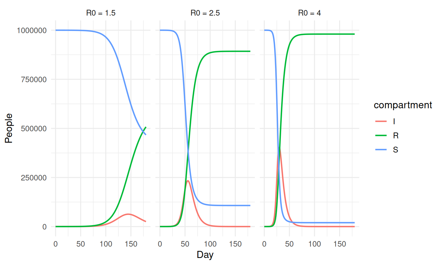
4. Check
Peak prevalence and attack rate should rise with R₀.
trajectories |>
  filter(compartment == "I") |>
  group_by(R0) |>
  summarise(peak_I = max(n), peak_day = time[which.max(n)]) |>
  arrange(R0)
# A tibble: 3 × 3
R0 peak_I peak_day
<dbl> <dbl> <dbl>
1 1.5 63023. 145
2 2.5 233307. 56
3 4 403070. 305. Report
An SIR compartmental model was simulated for a population of one million with a 7-day mean infectious period across three basic reproduction numbers (R₀ = 1.5, 2.5, 4). Peak prevalence and the final attack rate increased sharply with R₀, illustrating how small changes in transmission translate into large changes in epidemic size. Calibrated analogues of this model underpin much real-world outbreak forecasting.
Note that β and γ are not directly observed; they are inferred from case counts, and the uncertainty in R₀ propagates from that inference.
Common pitfalls
- Interpreting SIR trajectories as forecasts rather than scenarios.
- Forgetting that a constant β across time ignores interventions.
- Comparing peak prevalence across parameter settings without holding N and I₀ constant.
Further reading
- Keeling MJ, Rohani P. Modeling Infectious Diseases in Humans and Animals.
- Soetaert K et al. Solving Differential Equations in R.
Session info
sessionInfo()R version 4.5.2 (2025-10-31 ucrt)
Platform: x86_64-w64-mingw32/x64
Running under: Windows 11 x64 (build 26200)
Matrix products: default
LAPACK version 3.12.1
locale:
[1] LC_COLLATE=English_Germany.utf8 LC_CTYPE=English_Germany.utf8
[3] LC_MONETARY=English_Germany.utf8 LC_NUMERIC=C
[5] LC_TIME=English_Germany.utf8
time zone: Europe/Berlin
tzcode source: internal
attached base packages:
[1] stats graphics grDevices utils datasets methods base
other attached packages:
[1] deSolve_1.42 lubridate_1.9.5 forcats_1.0.1 stringr_1.6.0
[5] dplyr_1.2.1 purrr_1.2.2 readr_2.2.0 tidyr_1.3.2
[9] tibble_3.3.1 ggplot2_4.0.3 tidyverse_2.0.0
loaded via a namespace (and not attached):
[1] gtable_0.3.6 jsonlite_2.0.0 compiler_4.5.2 tidyselect_1.2.1
[5] scales_1.4.0 yaml_2.3.12 fastmap_1.2.0 R6_2.6.1
[9] labeling_0.4.3 generics_0.1.4 knitr_1.51 htmlwidgets_1.6.4
[13] pillar_1.11.1 RColorBrewer_1.1-3 tzdb_0.5.0 rlang_1.2.0
[17] stringi_1.8.7 xfun_0.57 S7_0.2.2 otel_0.2.0
[21] timechange_0.4.0 cli_3.6.6 withr_3.0.2 magrittr_2.0.4
[25] digest_0.6.39 grid_4.5.2 hms_1.1.4 lifecycle_1.0.5
[29] vctrs_0.7.3 evaluate_1.0.5 glue_1.8.1 farver_2.1.2
[33] rmarkdown_2.31 tools_4.5.2 pkgconfig_2.0.3 htmltools_0.5.9