library(tidyverse)
library(survival)
library(pROC)
set.seed(42)
theme_set(theme_minimal(base_size = 12))Week 3, Session 5 — Time-dependent Brier, IPA, external validation
Course 4 — #courses
Note
Testing labs use the main template: Hypothesis → Visualise → Assumptions → Conduct → Conclude.
Learning objectives
- Compute a time-dependent Brier score and the Index of Prediction Accuracy (IPA).
- Simulate an external-validation cohort with distribution shift and evaluate a fitted model on it.
- Describe why a model can have a high internal AUC and a bad external IPA.
Prerequisites
Survival ML from Session 4; calibration from Course 1.
Background
Validation is the point at which a prediction model either earns its keep or does not. Internal validation — CV or the bootstrap on the training data — controls optimism from the fitting step. External validation applies the fixed model to an independent cohort and measures discrimination, calibration, and clinical utility. Time- dependent Brier scores and IPA (1 − Brier/Brier_null) summarise the cost of a probabilistic prediction at a given horizon, combining discrimination and calibration into a single number per time.
Real biomedical models routinely lose performance on external cohorts. Changes in case mix, measurement, baseline risk, or predictor effects can affect performance in different ways. This lab changes the covariate distribution while keeping the conditional event model fixed.
TRIPOD-AI asks you to report all three — discrimination, calibration, clinical utility — on both internal and external data, and to disclose the shift between them. A reader who only sees AUC on internal data has no basis for deploying the model.
Setup
1. Hypothesis
A Cox model fit on a development cohort retains its calibration and discrimination on an external cohort with shifted covariate distribution.
2. Visualise
make_cohort <- function(n, mu_x = 0, beta = 0.6) {
  x <- rnorm(n, mu_x)
  lp <- beta * x
  t <- rexp(n, rate = exp(lp - 1))
  c <- rexp(n, rate = 0.1)
  time <- pmin(t, c)
  event <- as.integer(t <= c)
  tibble(x = x, time = time, event = event)
}
dev  <- make_cohort(500, mu_x = 0)
ext  <- make_cohort(500, mu_x = 1.0)   # distribution shift
bind_rows(dev |> mutate(cohort = "dev"),
          ext |> mutate(cohort = "ext")) |>
  ggplot(aes(x, fill = cohort)) +
  geom_histogram(bins = 30, alpha = 0.7, position = "identity")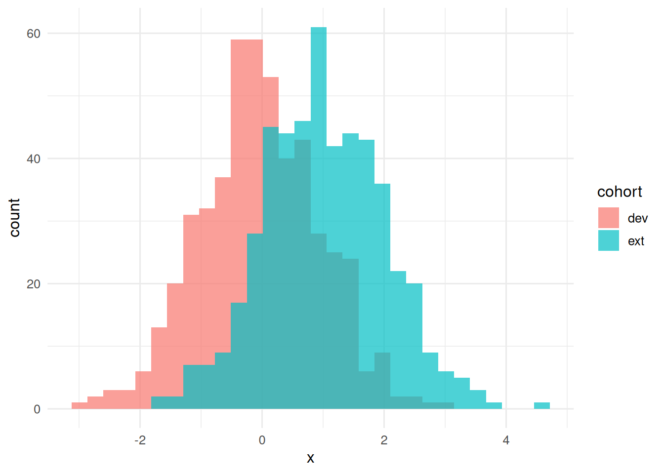
3. Assumptions
Censoring is independent of both event time and covariates in this simulation. We use marginal inverse-probability-of-censoring weights (IPCW), require positive censoring survival at the horizon, assume Cox proportional hazards, and use no time-varying covariates. Subjects censored before the horizon have unknown outcomes and are not coded as event-free.
4. Conduct
Fit on dev; predict survival at a fixed horizon on both cohorts.
fit <- coxph(Surv(time, event) ~ x, data = dev)
horizon <- 3

# Match the mean-centred baseline hazard to the same prediction reference.
# This helper is for the unstratified, fixed-covariate model used in this lab.
predict_surv <- function(fit, newdata, t) {
  bh <- basehaz(fit, centered = TRUE)
  stopifnot(length(t) == 1, is.finite(t), t >= 0, t <= max(bh$time))
  H0 <- c(0, bh$hazard)[findInterval(t, bh$time) + 1L]
  lp <- predict(fit, newdata = newdata, type = "lp", reference = "sample")
  exp(-H0 * exp(lp))
}

# Marginal IPCW is valid here because censoring is independent of X and T.
# Censoring that depends on predictors needs a conditional censoring model.
horizon_weights <- function(data, t) {
  g <- survfit(Surv(time, 1 - event) ~ 1, data = data)
  g_before <- c(1, g$surv)[findInterval(data$time, g$time, left.open = TRUE) + 1L]
  g_at <- c(1, g$surv)[findInterval(t, g$time) + 1L]
  cases <- data$event == 1 & data$time <= t
  controls <- data$time > t
  if (g_at <= 0 || any(g_before[cases] <= 0))
    stop("Insufficient censoring support at this horizon")
  weights <- numeric(nrow(data))
  weights[cases] <- 1 / g_before[cases]
  weights[controls] <- 1 / g_at
  list(cases = cases, controls = controls, weights = weights)
}

score_horizon <- function(data, p_event, t) {
  stopifnot(length(p_event) == nrow(data), all(is.finite(p_event)),
            all(p_event >= 0 & p_event <= 1))
  w <- horizon_weights(data, t)
  brier <- mean(w$weights * (as.numeric(w$cases) - p_event)^2)
  km <- survfit(Surv(time, event) ~ 1, data = data)
  null_risk <- 1 - c(1, km$surv)[findInterval(t, km$time) + 1L]
  null_brier <- mean(w$weights * (as.numeric(w$cases) - null_risk)^2)
  # Cumulative/dynamic AUC: observed cases by t against survivors beyond t.
  auc <- NA_real_
  if (any(w$cases) && any(w$controls)) {
    order_control <- order(p_event[w$controls])
    control_risk <- p_event[w$controls][order_control]
    cumulative_weight <- c(0, cumsum(w$weights[w$controls][order_control]))
    below <- cumulative_weight[findInterval(p_event[w$cases], control_risk,
                                           left.open = TRUE) + 1L]
    at_or_below <- cumulative_weight[findInterval(p_event[w$cases], control_risk) + 1L]
    auc <- sum(w$weights[w$cases] * (below + .5 * (at_or_below - below))) /
      (sum(w$weights[w$cases]) * sum(w$weights[w$controls]))
  }
  c(auc = auc, brier = brier,
    ipa = if (null_brier > 0) 1 - brier / null_brier else NA_real_)
}

s_dev <- predict_surv(fit, dev, horizon)
s_ext <- predict_surv(fit, ext, horizon)
metrics_dev <- score_horizon(dev, 1 - s_dev, horizon)
metrics_ext <- score_horizon(ext, 1 - s_ext, horizon)
b_dev <- unname(metrics_dev["brier"]); b_ext <- unname(metrics_ext["brier"])
ipa_dev <- unname(metrics_dev["ipa"]); ipa_ext <- unname(metrics_ext["ipa"])
auc_dev <- unname(metrics_dev["auc"]); auc_ext <- unname(metrics_ext["auc"])
rbind(development_apparent = metrics_dev, external = metrics_ext)
auc brier ipa
development_apparent 0.7606899 0.1909777 0.1791146
external 0.7399078 0.1375266 0.1099784A calibration plot at the horizon.
mk_cal <- function(p, data, lab, t) {
  breaks <- unique(quantile(p, seq(0, 1, by = .2)))
  bin <- if (length(breaks) > 1) cut(p, breaks, include.lowest = TRUE) else factor(rep(1, length(p)))
  bind_rows(lapply(split(seq_along(p), bin), function(i) {
    km <- survfit(Surv(time, event) ~ 1, data = data[i, ])
    # Do not extend a group's observed risk beyond its follow-up support.
    observed <- if (max(data$time[i]) >= t) {
      1 - c(1, km$surv)[findInterval(t, km$time) + 1L]
    } else NA_real_
    tibble(cohort = lab, mean_pred = mean(p[i]), obs = observed)
  }))
}
bind_rows(mk_cal(1 - s_dev, dev, "development (apparent)", horizon),
          mk_cal(1 - s_ext, ext, "external", horizon)) |>
  ggplot(aes(mean_pred, obs, colour = cohort)) +
  geom_point() + geom_line() +
  geom_abline(slope = 1, intercept = 0, colour = "grey50") +
  labs(x = "Predicted event probability at horizon",
       y = "Kaplan–Meier event probability within prediction groups")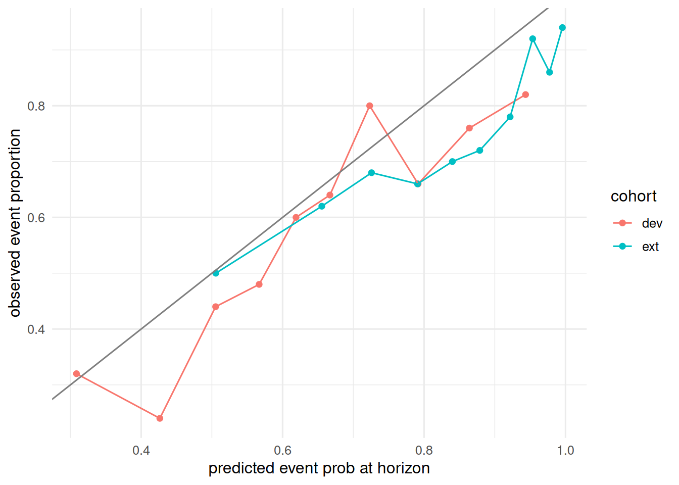
5. Concluding statement
At horizon 3, the independent simulated external cohort had cumulative/dynamic AUC 0.74, IPCW Brier score 0.138, and IPA 0.11. Apparent development values were AUC 0.76, Brier 0.191, and IPA 0.18. Development estimates reuse training data and therefore do not constitute internal validation.
Only the distribution of X changes here; the conditional event-time model is unchanged. Such covariate shift need not cause miscalibration. Brier, AUC, and the cohort-specific null model used for IPA may change with case mix even when predictions remain calibrated. The grouped calibration plot is descriptive and has sampling uncertainty; it does not establish a systematic direction of error in every simulation.
Mention that recalibration (update the baseline hazard or the intercept of a logistic model) often fixes calibration without retraining the whole model.
Common pitfalls
- Reporting AUC as the only discrimination metric on an external cohort.
- Ignoring censoring when computing a Brier score at a horizon;
pecorriskRegressionhandle this properly. - Recalibrating on external data and then reporting the resulting performance as external validation.
Further reading
- Graf E, Schmoor C, Sauerbrei W, Schumacher M (1999), Assessment and comparison of prognostic classification schemes for survival data.
- Kattan MW, Gerds TA (2018), The index of prediction accuracy: an intuitive measure useful for evaluating risk prediction models.
- Steyerberg EW, Clinical Prediction Models, ch. 15–17.
Session info
sessionInfo()R version 4.6.1 (2026-06-24)
Platform: x86_64-pc-linux-gnu
Running under: Ubuntu 26.04.1 LTS
Matrix products: default
BLAS: /usr/lib/x86_64-linux-gnu/openblas-pthread/libblas.so.3
LAPACK: /usr/lib/x86_64-linux-gnu/openblas-pthread/libopenblasp-r0.3.32.so; LAPACK version 3.12.0
locale:
[1] LC_CTYPE=C.UTF-8 LC_NUMERIC=C LC_TIME=C.UTF-8
[4] LC_COLLATE=C.UTF-8 LC_MONETARY=C.UTF-8 LC_MESSAGES=C.UTF-8
[7] LC_PAPER=C.UTF-8 LC_NAME=C LC_ADDRESS=C
[10] LC_TELEPHONE=C LC_MEASUREMENT=C.UTF-8 LC_IDENTIFICATION=C
time zone: UTC
tzcode source: system (glibc)
attached base packages:
[1] stats graphics grDevices datasets utils methods base
other attached packages:
[1] pROC_1.19.1 survival_3.8-6 lubridate_1.9.5 forcats_1.0.1
[5] stringr_1.6.0 dplyr_1.2.1 purrr_1.2.2 readr_2.2.0
[9] tidyr_1.3.2 tibble_3.3.1 ggplot2_4.0.3 tidyverse_2.0.0
loaded via a namespace (and not attached):
[1] Matrix_1.7-5 gtable_0.3.6 jsonlite_2.0.0 compiler_4.6.1
[5] renv_1.3.1 Rcpp_1.1.2 tidyselect_1.2.1 splines_4.6.1
[9] scales_1.4.0 yaml_2.3.12 fastmap_1.2.0 lattice_0.22-9
[13] R6_2.6.1 labeling_0.4.3 generics_0.1.4 knitr_1.52
[17] htmlwidgets_1.6.4 tzdb_0.5.0 pillar_1.11.1 RColorBrewer_1.1-3
[21] rlang_1.3.0 stringi_1.8.9 xfun_0.62 S7_0.2.2
[25] otel_0.2.0 timechange_0.4.0 cli_3.6.6 withr_3.0.3
[29] magrittr_2.0.5 digest_0.6.39 grid_4.6.1 hms_1.1.4
[33] lifecycle_1.0.5 vctrs_0.7.3 evaluate_1.0.5 glue_1.8.1
[37] farver_2.1.2 rmarkdown_2.32 tools_4.6.1 pkgconfig_2.0.3
[41] htmltools_0.5.9