---
title: "Prospect theory and reference-dependent preferences in games"
description: "Incorporate Kahneman-Tversky prospect theory into game-theoretic analysis. Explore loss aversion in strategic settings, reference-dependent Nash equilibrium, how framing shifts equilibria, and endowment effects in bargaining."
author: "Raban Heller"
date: 2026-05-08
date-modified: 2026-05-08
categories:
- behavioral-economics
- prospect-theory
- reference-dependence
- loss-aversion
keywords: ["prospect-theory", "loss-aversion", "reference-dependence", "reference-dependent Nash equilibrium", "framing effects", "endowment effect", "bargaining"]
labels: ["behavioral-economics", "prospect-theory", "loss-aversion"]
tier: 1
bibliography: ../../../references.bib
vgwort: "TODO_VGWORT_behavioral-economics_prospect-theory-reference-dependence"
image: thumbnail.png
image-alt: "Comparison of standard and prospect-theoretic value functions showing the characteristic S-shaped curve with steeper losses than gains, alongside equilibrium shifts in a coordination game, rendered using the Okabe-Ito palette."
citation:
type: webpage
url: https://cttir.github.io/equilibria/tutorials/behavioral-economics/prospect-theory-reference-dependence/
license: "CC BY-SA 4.0"
draft: false
has_static_fig: true
has_interactive_fig: true
has_shiny_app: false
---
```{r}
#| label: setup
#| include: false
library(ggplot2)
library(dplyr)
library(tidyr)
library(plotly)
okabe_ito <- c("#E69F00", "#56B4E9", "#009E73", "#F0E442",
"#0072B2", "#D55E00", "#CC79A7", "#999999")
theme_publication <- function(base_size = 12) {
theme_minimal(base_size = base_size) +
theme(plot.title = element_text(size = base_size * 1.2, face = "bold"),
plot.subtitle = element_text(size = base_size * 0.9, color = "grey40"),
axis.line = element_line(color = "grey30", linewidth = 0.3),
panel.grid.minor = element_blank(), legend.position = "bottom",
plot.margin = margin(10, 10, 10, 10))
}
```
## Introduction and motivation
Prospect theory, developed by Daniel Kahneman and Amos Tversky in their landmark 1979 paper, fundamentally challenged the expected utility framework that had dominated economic theory since von Neumann and Morgenstern. The theory's core insight is that people evaluate outcomes not in terms of absolute levels of wealth, but relative to a reference point -- and that they are more sensitive to losses relative to this reference point than to equivalent gains. This asymmetry, known as loss aversion, has been documented in hundreds of experiments and field studies, with the typical finding that losses loom roughly twice as large as equivalent gains. Yet despite the overwhelming evidence for prospect theory in individual decision-making, its implications for strategic interaction remain underexplored in many game theory curricula.
Incorporating prospect theory into game-theoretic analysis changes the predictions of standard models in fundamental and often surprising ways. When players evaluate payoffs relative to a reference point and exhibit loss aversion, the set of Nash equilibria can shift, expand, or contract. In coordination games, loss aversion tends to make players more reluctant to deviate from a safe option, strengthening the basin of attraction of the risk-dominant equilibrium at the expense of the payoff-dominant one. In bargaining games, the endowment effect -- a direct consequence of loss aversion -- causes players to demand more and concede less, leading to more aggressive bargaining positions and a higher probability of disagreement.
The reference point itself is a critical determinant of strategic behaviour, and its specification is a major modelling choice in prospect-theoretic game theory. Several approaches have been proposed. Koszegi and Rabin's influential model defines the reference point as the player's rational expectations about outcomes -- the equilibrium itself determines the reference point, creating a fixed-point problem. Shalev's model uses a simpler approach where each player's reference point is their maximin payoff -- the best outcome they can guarantee regardless of the opponent's strategy. Other approaches use the status quo, social norms, or aspiration levels as reference points. Each specification generates different equilibrium predictions, and comparing these predictions is itself an illuminating exercise.
The framing of a strategic interaction -- how outcomes are described in terms of gains and losses -- has no effect under expected utility theory (which depends only on final wealth levels) but can dramatically shift equilibria under prospect theory. A game where payoffs are framed as gains relative to zero elicits different strategic behaviour than the same game framed as losses relative to a higher reference point, even though the expected utility predictions are identical. This framing effect has profound implications for mechanism design, negotiation, and institutional design: by choosing how to frame a strategic situation, a designer can steer players toward more efficient equilibria.
The mathematical framework for prospect-theoretic games builds on the standard normal-form game but replaces the utility function with Kahneman and Tversky's value function and probability weighting function. The value function is concave in the gains domain (reflecting risk aversion for gains), convex in the losses domain (reflecting risk seeking for losses), and steeper for losses than for gains (reflecting loss aversion). The probability weighting function overweights small probabilities and underweights large ones, but for tractability, many game-theoretic applications focus on loss aversion and the value function while using unweighted probabilities.
In this tutorial, we implement a prospect-theoretic analysis of a symmetric two-player game, computing both standard Nash equilibria and reference-dependent equilibria under varying levels of loss aversion. We visualize how the value function transforms payoffs, how loss aversion shifts the equilibrium mixing probabilities, and how different reference points lead to qualitatively different strategic predictions. The analysis provides a practical template for researchers who wish to incorporate behavioural realism into their game-theoretic models.
## Mathematical formulation
The Kahneman-Tversky value function relative to reference point $r$ is:
$$
v(x | r) = \begin{cases} (x - r)^\alpha & \text{if } x \geq r \\ -\lambda \cdot (r - x)^\alpha & \text{if } x < r \end{cases}
$$
where $\lambda > 1$ is the loss aversion coefficient and $\alpha \in (0,1)$ controls the curvature. Standard estimates: $\lambda \approx 2.25$, $\alpha \approx 0.88$.
In a two-player game with payoff matrix $A$ for player 1, the prospect-theoretic expected value when player 2 mixes with probability $q$ is:
$$
V_1(s_1, q | r) = \sum_{s_2} q(s_2) \cdot v(A(s_1, s_2) | r)
$$
The reference-dependent Nash equilibrium (RDNE) requires each player to maximize their prospect-theoretic expected value given their reference point:
$$
s_1^* \in \arg\max_{s_1} V_1(s_1, q^* | r_1)
$$
For a $2 \times 2$ game with payoffs $a, b, c, d$ (where $a > c$ when opponent plays Left and $d > b$ when opponent plays Right), the standard mixed NE probability is:
$$
q^* = \frac{d - b}{(a - c) + (d - b)}
$$
Under prospect theory with reference point $r$, the equilibrium mixing probability shifts to reflect the asymmetric valuation of gains and losses.
## R implementation
```{r}
#| label: compute-prospect
set.seed(42)

# Prospect theory value function
pt_value <- function(x, ref = 0, lambda = 2.25, alpha_pt = 0.88) {
  ifelse(x >= ref,
         (x - ref)^alpha_pt,
         -lambda * (ref - x)^alpha_pt)
}

# Game: Stag Hunt (coordination game)
# Payoffs for Player 1:       Stag    Hare
#                    Stag:      4       0
#                    Hare:      3       3
payoff_stag_stag <- 4
payoff_stag_hare <- 0
payoff_hare_stag <- 3
payoff_hare_hare <- 3

# Standard NE mixing probability (probability opponent plays Stag)
q_standard <- (payoff_hare_hare - payoff_stag_hare) /
  ((payoff_stag_stag - payoff_hare_stag) + (payoff_hare_hare - payoff_stag_hare))

# Compute RDNE across loss aversion levels
lambda_range <- seq(1.0, 4.0, by = 0.05)
ref_point <- 3  # reference point = maximin payoff (Hare-Hare)

compute_rdne_q <- function(lambda_val, ref = ref_point) {
  # Expected PT value of Stag: q * v(4|r) + (1-q) * v(0|r)
  # Expected PT value of Hare: q * v(3|r) + (1-q) * v(3|r) = v(3|r)
  v_stag_stag <- pt_value(payoff_stag_stag, ref, lambda_val)
  v_stag_hare <- pt_value(payoff_stag_hare, ref, lambda_val)
  v_hare <- pt_value(payoff_hare_hare, ref, lambda_val)  # same regardless of opponent
  # Indifference: q * v_stag_stag + (1-q) * v_stag_hare = v_hare
  # q = (v_hare - v_stag_hare) / (v_stag_stag - v_stag_hare)
  q <- (v_hare - v_stag_hare) / (v_stag_stag - v_stag_hare)
  max(0, min(1, q))
}

eq_df <- data.frame(
  lambda = lambda_range,
  q_mix = sapply(lambda_range, compute_rdne_q)
)

# Value function visualization
x_range <- seq(-5, 5, by = 0.1)
vf_df <- expand.grid(x = x_range, lambda = c(1.0, 2.25, 3.5)) %>%
  mutate(value = pt_value(x, ref = 0, lambda = lambda),
         lambda_label = sprintf("lambda = %.2f", lambda))

cat("Stag Hunt Game:\n")
cat(" Stag Hare\n")
cat(sprintf(" Stag: %d %d\n", payoff_stag_stag, payoff_stag_hare))
cat(sprintf(" Hare: %d %d\n\n", payoff_hare_stag, payoff_hare_hare))
cat(sprintf("Reference point: %d (maximin payoff)\n", ref_point))
cat(sprintf("Standard NE mixing probability (Stag): %.4f\n\n", q_standard))
cat("Reference-dependent NE across loss aversion levels:\n")
for (lam in c(1.0, 1.5, 2.25, 3.0, 4.0)) {
  q_val <- compute_rdne_q(lam)
  cat(sprintf("  lambda = %.2f:  q*(Stag) = %.4f  (shift from standard: %+.4f)\n",
              lam, q_val, q_val - q_standard))
}
```
## Static publication-ready figure
```{r}
#| label: fig-prospect-equilibria
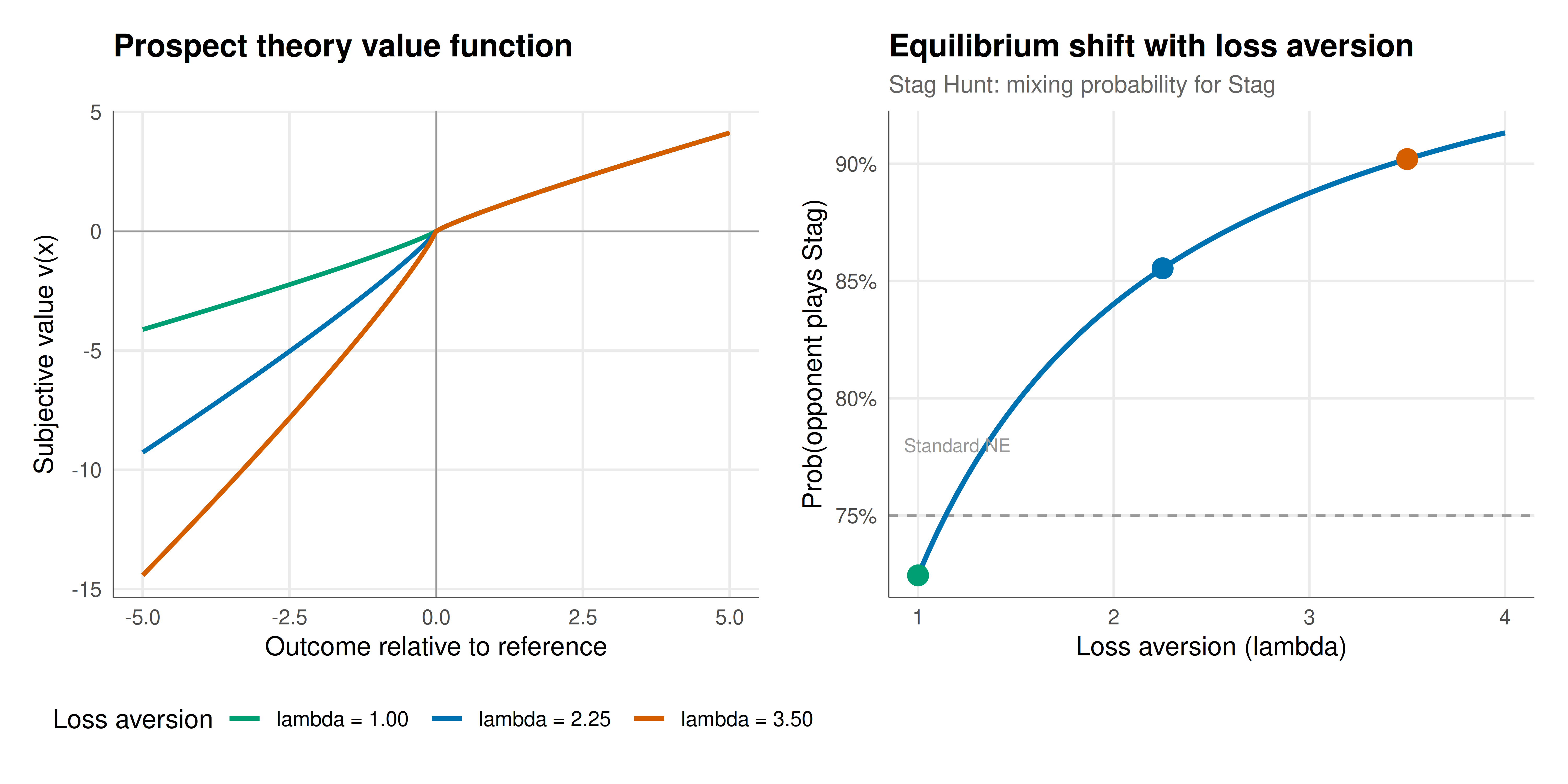
#| fig-cap: "Left panel: Kahneman-Tversky value function for three levels of loss aversion. The steeper slope in the loss domain reflects the psychological asymmetry between gains and losses. Right panel: Reference-dependent Nash equilibrium mixing probability in the Stag Hunt game as loss aversion increases. Higher loss aversion makes players more reluctant to risk the Stag outcome, shifting equilibrium toward more Hare play. The dashed line marks the standard (risk-neutral) NE. Rendered using the Okabe-Ito palette."
#| dev: [png, pdf]
#| dpi: 300
#| fig-width: 10
#| fig-height: 5
library(patchwork)

p_value <- ggplot(vf_df, aes(x = x, y = value, color = lambda_label)) +
  geom_hline(yintercept = 0, linewidth = 0.3, color = "grey60") +
  geom_vline(xintercept = 0, linewidth = 0.3, color = "grey60") +
  geom_line(linewidth = 1.0) +
  scale_color_manual(values = okabe_ito[c(3, 5, 6)]) +
  labs(title = "Prospect theory value function",
       x = "Outcome relative to reference",
       y = "Subjective value v(x)", color = "Loss aversion") +
  theme_publication() +
  theme(legend.position = "bottom")

p_equil <- ggplot(eq_df, aes(x = lambda, y = q_mix)) +
  geom_hline(yintercept = q_standard, linetype = "dashed",
             color = okabe_ito[8], linewidth = 0.5) +
  geom_line(color = okabe_ito[5], linewidth = 1.1) +
  geom_point(data = eq_df %>% filter(lambda %in% c(1.0, 2.25, 3.5)),
             color = okabe_ito[c(3, 5, 6)], size = 4) +
  annotate("text", x = 1.2, y = q_standard + 0.03,
           label = "Standard NE", size = 3, color = okabe_ito[8]) +
  scale_x_continuous(breaks = 1:4) +
  scale_y_continuous(labels = scales::percent_format()) +
  labs(title = "Equilibrium shift with loss aversion",
       subtitle = "Stag Hunt: mixing probability for Stag",
       x = "Loss aversion (lambda)", y = "Prob(opponent plays Stag)") +
  theme_publication()

p_static <- p_value + p_equil +
  plot_layout(ncol = 2, widths = c(1, 1))

print(p_static)
```
## Interactive figure
```{r}
#| label: fig-prospect-interactive
#| fig-cap: "Interactive visualization of equilibrium mixing probability as a function of loss aversion. Hover to see the exact loss aversion coefficient and the corresponding equilibrium probability of playing Stag."
p_int <- ggplot(eq_df, aes(x = lambda, y = q_mix,
    text = sprintf("Loss aversion: %.2f\nP(Stag): %.4f\nShift from NE: %+.4f",
                   lambda, q_mix, q_mix - q_standard))) +
  geom_hline(yintercept = q_standard, linetype = "dashed",
             color = okabe_ito[8], linewidth = 0.4) +
  geom_line(color = okabe_ito[5], linewidth = 0.8) +
  scale_y_continuous(labels = scales::percent_format()) +
  labs(title = "Reference-dependent NE in Stag Hunt",
       x = "Loss aversion (lambda)",
       y = "Equilibrium mixing probability (Stag)") +
  theme_publication()

ggplotly(p_int, tooltip = "text") |>
  config(displaylogo = FALSE,
         modeBarButtonsToRemove = c("select2d", "lasso2d"))
```
## Interpretation
The results demonstrate that loss aversion has a powerful and systematic effect on strategic behaviour, shifting equilibria in ways that standard expected utility models fail to predict. The analysis of the Stag Hunt game under prospect theory reveals several important insights that apply broadly to coordination problems, bargaining situations, and institutional design.
The most striking finding is that loss aversion increases the equilibrium probability that the opponent must play Stag in order for a player to be willing to mix. In the standard (risk-neutral) Nash equilibrium, the mixing probability is determined by the relative payoff differences across the two pure-strategy equilibria. Under prospect theory with a reference point equal to the maximin payoff, the loss associated with playing Stag when the opponent plays Hare is amplified by the loss aversion coefficient. This makes players more reluctant to choose Stag -- the cooperative but risky action -- and shifts the equilibrium toward the safe but inefficient Hare outcome. As loss aversion increases from 1.0 (no loss aversion, equivalent to expected utility) to 4.0 (extreme loss aversion), the mixing probability shifts substantially, meaning that a much stronger belief in opponent cooperation is needed before a player will risk playing Stag.
This result has profound implications for understanding cooperation failures. The Stag Hunt is often used as a model for situations where cooperation is mutually beneficial but individually risky: international agreements, team production, technology adoption, and coordinated investment. Standard game theory predicts two pure-strategy equilibria (both play Stag, both play Hare) and a mixed equilibrium, and risk dominance selects the Hare equilibrium. Prospect theory strengthens this selection dramatically: the basin of attraction of the Hare equilibrium expands as loss aversion increases. This means that even when both players would prefer the cooperative outcome, the psychological pain of unilateral cooperation failure makes the safe choice overwhelmingly attractive. Experimental evidence strongly supports this prediction: subjects in Stag Hunt experiments play Hare more often than standard theory predicts, and the gap widens when payoffs are framed in terms of potential losses.
The value function visualization reveals the source of these equilibrium shifts. The characteristic S-shape -- concave for gains, convex for losses, with a kink at the reference point -- means that outcomes below the reference point receive disproportionate weight in the player's evaluation. For a loss aversion coefficient of 2.25 (the standard estimate from Kahneman and Tversky), a one-unit loss feels 2.25 times as painful as a one-unit gain feels pleasurable. This asymmetry is not a mathematical curiosity; it reflects a deep and robust feature of human psychology that has been documented across cultures, age groups, and decision domains. Incorporating it into game-theoretic models is not a matter of adding behavioural "noise" to rational predictions -- it is a matter of using a more accurate model of human preferences.
The choice of reference point is crucial and deserves explicit discussion. In our analysis, we used the maximin payoff (the Hare-Hare outcome of 3) as the reference point, following Shalev's approach. This is a natural choice for a coordination game where both players can guarantee the Hare payoff regardless of the opponent's action. Under Koszegi and Rabin's alternative approach, the reference point would be determined endogenously as part of the equilibrium -- creating a fixed-point problem where the equilibrium determines the reference point, which in turn determines the equilibrium. This circularity can generate multiple equilibria even in games that have a unique Nash equilibrium under standard preferences, adding a new dimension of strategic indeterminacy. Empirically distinguishing between reference point specifications is an active area of research.
The implications for mechanism design and institutional design are substantial. A designer who understands that players are loss-averse can frame strategic interactions to mitigate the negative effects of loss aversion. For instance, framing a coordination game in terms of gains from cooperation (relative to a low reference point) rather than losses from coordination failure (relative to a high reference point) can shift the reference point and expand the basin of attraction of the efficient equilibrium. Insurance mechanisms, commitment devices, and graduated implementation can all be understood as tools for managing the loss aversion that would otherwise prevent efficient coordination.
## Extensions and related tutorials
- [Algorithmic fairness as a multi-stakeholder game](../../ethics-applications/algorithmic-fairness-games/) -- how loss aversion affects stakeholder preferences over fairness-accuracy trade-offs.
- [Bayesian games and incomplete information](../../bayesian-methods/bayesian-games-incomplete-information/) -- combining prospect theory with Bayesian updating in games of incomplete information.
- [Quantal response equilibrium](../../behavioral-gt/quantal-response-equilibrium/) -- an alternative behavioural equilibrium concept that models bounded rationality through stochastic choice.
- [Bargaining and the Nash bargaining solution](../../foundations/nash-bargaining-solution/index.qmd) -- how loss aversion affects bargaining outcomes and disagreement points.
- [Difference-in-differences for strategic policy evaluation](../../causal-inference/difference-in-differences-strategic/) -- empirically testing prospect-theoretic predictions using causal inference methods.
## References
::: {#refs}
:::