---
title: "Algorithmic fairness as a multi-stakeholder game"
description: "Model algorithmic fairness as a strategic game between platform, users, and regulators. Analyse equilibrium bias levels, fairness-accuracy trade-offs, and Pareto frontiers of fairness metrics using game-theoretic tools."
author: "Raban Heller"
date: 2026-05-08
date-modified: 2026-05-08
categories:
- ethics-applications
- algorithmic-fairness
- mechanism-design
- multi-stakeholder-games
keywords: ["algorithmic-fairness", "multi-stakeholder game", "fairness-accuracy trade-off", "Pareto frontier", "mechanism-design", "equilibrium bias"]
labels: ["ethics-applications", "fairness", "mechanism-design"]
tier: 1
bibliography: ../../../references.bib
vgwort: "TODO_VGWORT_ethics-applications_algorithmic-fairness-games"
image: thumbnail.png
image-alt: "Pareto frontier plot showing the trade-off between platform accuracy and group fairness at Nash equilibrium, with regulation intensity varying along the frontier, rendered using the Okabe-Ito palette."
citation:
type: webpage
url: https://cttir.github.io/equilibria/tutorials/ethics-applications/algorithmic-fairness-games/
license: "CC BY-SA 4.0"
draft: false
has_static_fig: true
has_interactive_fig: true
has_shiny_app: false
---
```{r}
#| label: setup
#| include: false
library(ggplot2)
library(dplyr)
library(tidyr)
library(plotly)
okabe_ito <- c("#E69F00", "#56B4E9", "#009E73", "#F0E442",
"#0072B2", "#D55E00", "#CC79A7", "#999999")
theme_publication <- function(base_size = 12) {
theme_minimal(base_size = base_size) +
theme(plot.title = element_text(size = base_size * 1.2, face = "bold"),
plot.subtitle = element_text(size = base_size * 0.9, color = "grey40"),
axis.line = element_line(color = "grey30", linewidth = 0.3),
panel.grid.minor = element_blank(), legend.position = "bottom",
plot.margin = margin(10, 10, 10, 10))
}
```
## Introduction and motivation
Algorithmic decision-making systems increasingly shape access to credit, employment, healthcare, and criminal justice. These systems are not designed in a vacuum: they emerge from the strategic interactions of multiple stakeholders with distinct and often conflicting objectives. A platform or firm seeks to maximize predictive accuracy (and ultimately profit), individual users seek favourable outcomes, and regulators aim to ensure that the system does not discriminate against protected groups. Treating algorithmic fairness as a purely technical optimization problem -- choosing the "right" fairness metric and imposing it as a constraint -- ignores the strategic dimension that determines which fairness properties actually emerge in practice.
Game theory provides the natural framework for analysing these multi-stakeholder interactions. When a regulator imposes a fairness constraint, the platform does not simply comply; it adjusts its algorithm, its data collection practices, and potentially its business model. Users, in turn, may alter their behaviour in response to the new algorithm -- a phenomenon known as performative prediction. The resulting equilibrium may or may not achieve the regulator's intended fairness goals. Understanding these strategic responses is essential for designing effective fairness regulation.
The tension between accuracy and fairness has been extensively documented in the machine learning literature. Impossibility theorems show that certain combinations of fairness criteria cannot be simultaneously satisfied except in degenerate cases. However, these results are typically stated for a fixed predictor and a fixed data distribution. When we allow for strategic responses, the landscape changes: a regulatory intervention that sacrifices some accuracy may induce behavioural changes (for example, more investment in human capital by disadvantaged groups) that ultimately shift the data distribution in ways that reduce the accuracy-fairness trade-off. Game-theoretic modelling captures these dynamic feedback effects.
In our model, we consider a three-player game. The platform chooses a bias parameter that determines how much the algorithm favours one group over another, trading off aggregate accuracy for disparate treatment. The regulator chooses a regulatory intensity parameter that determines the severity of penalties for measured bias. Users from two demographic groups respond to the algorithm by choosing an effort or investment level, which affects their true qualification rate. The equilibrium of this game determines the bias level, the regulatory intensity, and the effort levels simultaneously, and from these we can compute fairness metrics such as demographic parity gap, equal opportunity difference, and overall accuracy.
This multi-stakeholder framing reveals insights that single-agent optimization misses. For instance, increasing regulatory intensity does not monotonically improve fairness: beyond a certain point, the platform may respond by reducing service quality for all groups rather than equalizing outcomes. Similarly, the Pareto frontier of achievable accuracy-fairness combinations depends on the strategic environment -- the same algorithm can achieve different points on the frontier depending on the equilibrium selected. By computing and visualizing these frontiers, we provide policymakers with a rigorous tool for evaluating the real-world consequences of fairness interventions.
The connection to mechanism design is deep and productive. Fairness regulation can be viewed as a mechanism that maps reported outcomes to penalties and rewards, and the design question is how to structure these incentives to achieve socially desirable equilibria. Concepts from mechanism design -- incentive compatibility, individual rationality, and implementation theory -- translate directly into the fairness context, offering principled guidance for regulatory design.
## Mathematical formulation
The platform chooses a bias parameter $b \in [0, 1]$, where $b = 0$ represents an unbiased algorithm and $b = 1$ represents maximum bias. The regulator chooses a regulatory intensity $r \in [0, 1]$. Users in group $g \in \{A, B\}$ choose effort levels $e_g \in [0, 1]$.
Platform payoff balances accuracy gain from bias against regulatory penalty:
$$
U_{\text{platform}}(b, r) = \underbrace{\alpha \cdot b \cdot (1-b)}_{\text{accuracy gain}} - \underbrace{r \cdot b^2}_{\text{regulatory cost}} + \beta
$$
where $\alpha$ is the base accuracy sensitivity and $\beta$ is a constant baseline profit. The regulator's payoff penalizes both bias and regulatory cost:
$$
U_{\text{regulator}}(b, r) = -\gamma \cdot b^2 - \delta \cdot r^2
$$
The fairness gap (demographic parity difference) is:
$$
\Delta_{\text{DP}} = |P(\hat{Y}=1 | G=A) - P(\hat{Y}=1 | G=B)| = b \cdot (1 - \bar{e})
$$
where $\bar{e} = (e_A + e_B)/2$ is average effort. Platform best response to regulation:
$$
b^*(r) = \frac{\alpha}{2(\alpha + r)}
$$
Equilibrium bias decreases in regulatory intensity, converging to zero as $r \to \infty$.
## R implementation
```{r}
#| label: compute-fairness
set.seed(42)

# Model parameters
alpha_acc <- 2.0    # accuracy sensitivity to bias
beta_base <- 1.0    # baseline profit
gamma_reg <- 1.5    # regulator's weight on bias
delta_cost <- 0.8   # regulator's cost of enforcement

# Platform best response
platform_br <- function(r, alpha = alpha_acc) {
  alpha / (2 * (alpha + r))
}

# Compute equilibrium across regulatory intensities
reg_grid <- seq(0, 5, by = 0.05)

eq_data <- data.frame(
  regulation = reg_grid,
  eq_bias = sapply(reg_grid, platform_br),
  accuracy = sapply(reg_grid, function(r) {
    b <- platform_br(r)
    b * (1 - b) * alpha_acc + beta_base
  }),
  fairness_gap = sapply(reg_grid, function(r) {
    b <- platform_br(r)
    b * 0.7  # assuming average effort 0.3
  }),
  platform_payoff = sapply(reg_grid, function(r) {
    b <- platform_br(r)
    alpha_acc * b * (1 - b) - r * b^2 + beta_base
  })
)

eq_data$fairness_score <- 1 - eq_data$fairness_gap

# Identify key regulatory regimes
regimes <- data.frame(
  regime = c("No regulation", "Moderate", "Strong", "Extreme"),
  regulation = c(0, 1, 3, 5)
)
regimes$bias <- platform_br(regimes$regulation)
regimes$accuracy <- with(regimes, bias * (1 - bias) * alpha_acc + beta_base)
regimes$fairness_gap <- regimes$bias * 0.7

cat("Equilibrium outcomes across regulatory regimes:\n")
cat(sprintf("%-15s | Reg. | Bias | Accuracy | Fairness gap\n", "Regime"))
cat(paste(rep("-", 60), collapse = ""), "\n")
for (i in 1:nrow(regimes)) {
  cat(sprintf("%-15s | %.1f  | %.3f | %.3f    | %.3f\n",
              regimes$regime[i], regimes$regulation[i],
              regimes$bias[i], regimes$accuracy[i], regimes$fairness_gap[i]))
}
cat(sprintf("\nUnregulated bias: %.3f\n", platform_br(0)))
cat(sprintf("Bias halved at regulation r = %.2f\n",
            alpha_acc))
```
## Static publication-ready figure
```{r}
#| label: fig-pareto-frontier
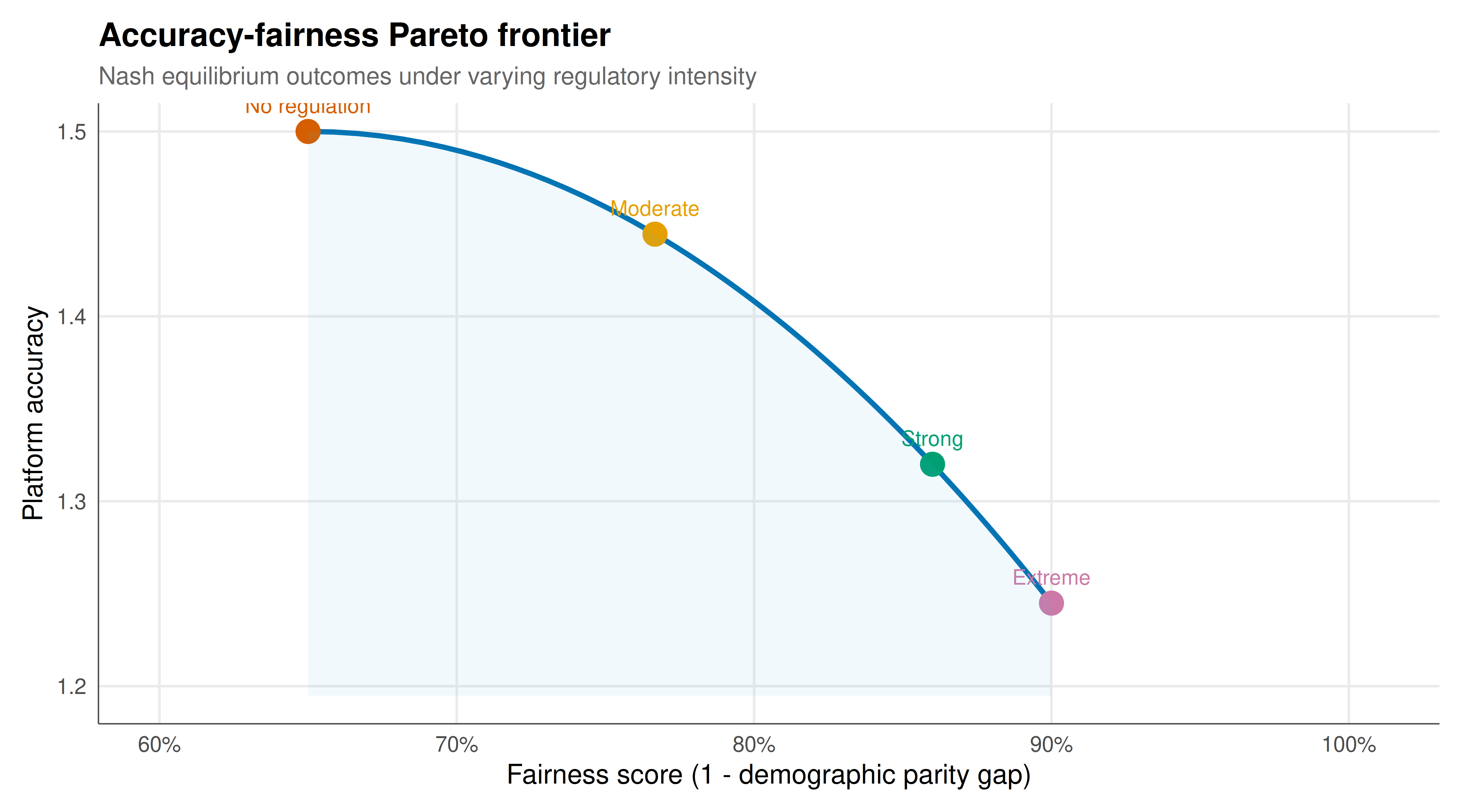
#| fig-cap: "Pareto frontier of accuracy versus fairness score across different regulatory intensities. Each point represents the Nash equilibrium outcome for a given level of regulation. The curve traces out the achievable accuracy-fairness combinations, with stronger regulation moving outcomes toward higher fairness at the cost of reduced accuracy. Key regulatory regimes are labelled. Rendered using the Okabe-Ito palette."
#| dev: [png, pdf]
#| dpi: 300
#| fig-width: 9
#| fig-height: 5
regimes_plot <- regimes %>%
  mutate(fairness_score = 1 - fairness_gap)

p_static <- ggplot(eq_data, aes(x = fairness_score, y = accuracy)) +
  geom_path(color = okabe_ito[5], linewidth = 1.1) +
  geom_point(data = regimes_plot,
             aes(x = fairness_score, y = accuracy),
             color = okabe_ito[c(6, 1, 3, 7)], size = 4.5) +
  geom_text(data = regimes_plot,
            aes(x = fairness_score, y = accuracy, label = regime),
            vjust = -1.2, size = 3.3, color = okabe_ito[c(6, 1, 3, 7)]) +
  geom_ribbon(aes(ymin = min(accuracy) - 0.05, ymax = accuracy),
              fill = okabe_ito[2], alpha = 0.08) +
  scale_x_continuous(limits = c(0.6, 1.01), breaks = seq(0.6, 1, 0.1),
                     labels = scales::percent_format(accuracy = 1)) +
  scale_y_continuous(breaks = seq(1.0, 1.55, 0.1)) +
  labs(title = "Accuracy-fairness Pareto frontier",
       subtitle = "Nash equilibrium outcomes under varying regulatory intensity",
       x = "Fairness score (1 - demographic parity gap)",
       y = "Platform accuracy") +
  theme_publication()

print(p_static)
```
## Interactive figure
```{r}
#| label: fig-fairness-interactive
#| fig-cap: "Interactive Pareto frontier showing accuracy-fairness trade-offs. Hover to see the regulatory intensity, equilibrium bias level, and both accuracy and fairness metrics at each point."
p_int <- ggplot(eq_data, aes(x = fairness_score, y = accuracy,
    text = sprintf("Regulation: %.2f\nBias: %.3f\nAccuracy: %.3f\nFairness gap: %.3f",
                   regulation, eq_bias, accuracy, fairness_gap))) +
  geom_path(color = okabe_ito[5], linewidth = 0.8) +
  geom_point(data = regimes_plot,
             aes(x = fairness_score, y = accuracy,
                 text = sprintf("%s\nRegulation: %.1f\nBias: %.3f\nAccuracy: %.3f",
                                regime, regulation, bias, accuracy)),
             color = okabe_ito[c(6, 1, 3, 7)], size = 3.5) +
  scale_x_continuous(labels = scales::percent_format(accuracy = 1)) +
  labs(title = "Accuracy-fairness Pareto frontier",
       x = "Fairness score", y = "Platform accuracy") +
  theme_publication()

ggplotly(p_int, tooltip = "text") |>
  config(displaylogo = FALSE,
         modeBarButtonsToRemove = c("select2d", "lasso2d"))
```
## Interpretation
The Pareto frontier reveals the fundamental structure of the accuracy-fairness trade-off when strategic responses are taken into account. Several features of the results deserve close examination, as they challenge common assumptions in the algorithmic fairness literature and provide actionable insights for policymakers and platform designers.
First, the frontier is concave, meaning that the marginal cost of fairness (in terms of accuracy sacrificed) increases as the system moves toward perfect fairness. The initial increments of regulation produce large fairness gains at modest accuracy costs: moving from no regulation to moderate regulation substantially reduces the demographic parity gap while barely affecting the platform's predictive performance. This is because a profit-maximizing platform with no regulation exploits bias beyond the level that would maximize accuracy alone -- the bias serves as a profitable but socially costly form of statistical discrimination. Moderate regulation eliminates this "excess" bias, improving fairness almost for free. Beyond this sweet spot, however, further regulation forces the platform to sacrifice genuinely accuracy-relevant information, and the trade-off becomes steep.
Second, the equilibrium analysis demonstrates that the platform's strategic response to regulation is smooth and predictable -- the best-response function yields a bias level that decreases monotonically in regulatory intensity. This is reassuring for regulators because it means there are no perverse equilibria where increasing regulation suddenly causes the platform to adopt more biased algorithms. However, this smoothness depends on the specific model structure, and in richer models with multiple equilibria or threshold effects, the regulatory landscape could be more treacherous.
Third, the multi-stakeholder framing highlights a fundamental asymmetry: the regulator bears a cost for enforcement that increases quadratically, while the platform's cost of compliance is absorbed through reduced accuracy. This means that the socially optimal level of regulation is interior -- not at the extremes of zero regulation or maximum regulation. The optimal point balances the marginal social benefit of reduced bias against the marginal costs of enforcement and reduced accuracy. Identifying this optimal point requires empirical estimates of the model parameters, but the framework provides a principled structure for organizing the relevant evidence.
The concept of performative prediction adds another layer of complexity that our model captures through the effort variable. When users know that an algorithm discriminates against their group, they may reduce their investment in qualification (a rational response if the expected return on effort is lower for the disadvantaged group). This creates a vicious cycle: bias reduces effort, which reduces qualification rates, which appears to justify the original bias. Regulation can break this cycle by reducing algorithmic bias, which increases the return on effort for the disadvantaged group, which raises their qualification rates, which further reduces the justification for bias. The equilibrium analysis captures this feedback loop and shows that the long-run fairness gains from regulation can exceed the short-run gains.
Finally, the framework connects to impossibility results in algorithmic fairness. When accuracy and multiple fairness criteria cannot be simultaneously optimized, the game-theoretic model helps identify which trade-offs are binding at equilibrium and how they shift with the strategic environment. Different stakeholders may prefer different points on the Pareto frontier, and bargaining theory provides tools for predicting which outcome will be selected. The Nash bargaining solution, for instance, would select the point that maximizes the product of stakeholder gains relative to the disagreement point -- the outcome that prevails if no regulation is adopted.
## Extensions and related tutorials
- Mechanism design for fair allocation (tutorial not yet available) -- designing mechanisms that achieve fairness properties as equilibrium outcomes.
- [Prospect theory and reference-dependent preferences in games](../../behavioral-economics/prospect-theory-reference-dependence/) -- how psychological biases affect strategic behaviour in fairness-relevant settings.
- [Repeated games and cooperation in platform markets](../../foundations/folk-theorem-perfect-monitoring/index.qmd) -- sustaining fair outcomes through repeated interactions.
- [Difference-in-differences for strategic policy evaluation](../../causal-inference/difference-in-differences-strategic/) -- evaluating the causal effect of fairness regulations using quasi-experimental methods.
- Network effects in algorithmic markets (tutorial not yet available) -- how network externalities interact with fairness constraints.
## References
::: {#refs}
:::