---
title: "Ultimatum game experiments and fairness norms"
description: "Analyse ultimatum game experimental data in R, compare observed behaviour with the subgame-perfect prediction, implement fairness utility models (Fehr-Schmidt, Bolton-Ockenfels), and visualise how culture, stakes, and framing affect offers and rejection thresholds."
author: "Raban Heller"
date: 2026-05-08
date-modified: 2026-05-08
categories:
- experimental-economics
- ultimatum-game
- fairness
- behavioral-game-theory
keywords: ["ultimatum game", "fairness norms", "rejection threshold", "Fehr-Schmidt", "experimental economics"]
labels: ["experiments", "behavioral-gt"]
tier: 1
bibliography: ../../../references.bib
vgwort: "TODO_VGWORT_experimental-economics_ultimatum-game-experiments"
image: thumbnail.png
image-alt: "Distribution of ultimatum game offers showing the modal offer at 40-50% of the pie, far above the subgame-perfect prediction of near-zero"
citation:
type: webpage
url: https://cttir.github.io/equilibria/tutorials/experimental-economics/ultimatum-game-experiments/
license: "CC BY-SA 4.0"
draft: false
has_static_fig: true
has_interactive_fig: true
has_shiny_app: false
---
```{r}
#| label: setup
#| include: false
library(ggplot2)
library(dplyr)
library(tidyr)
library(plotly)
okabe_ito <- c("#E69F00", "#56B4E9", "#009E73", "#F0E442",
"#0072B2", "#D55E00", "#CC79A7", "#999999")
theme_publication <- function(base_size = 12) {
theme_minimal(base_size = base_size) +
theme(plot.title = element_text(size = base_size * 1.2, face = "bold"),
plot.subtitle = element_text(size = base_size * 0.9, color = "grey40"),
axis.line = element_line(color = "grey30", linewidth = 0.3),
panel.grid.minor = element_blank(), legend.position = "bottom",
plot.margin = margin(10, 10, 10, 10))
}
```
## Introduction & motivation
The ultimatum game is perhaps the most famous experiment in behavioural economics. The rules are simple: a proposer divides a fixed sum (say, $10) between themselves and a responder; the responder can accept (both get the proposed split) or reject (both get nothing). The subgame-perfect equilibrium prediction is stark: the proposer offers the smallest positive amount, and the responder accepts any positive offer, since something is better than nothing. Yet decades of experimental evidence from dozens of countries show that modal offers cluster around 40-50% of the pie, and offers below 20% are rejected roughly half the time.
This dramatic failure of standard theory has profound implications. It demonstrates that fairness, reciprocity, and social norms are powerful forces in human decision-making that cannot be dismissed as noise or confusion. The robustness of the finding — it replicates across cultures, stake sizes (up to several months' wages), and framings — suggests that preferences over fairness are a fundamental feature of human psychology, not an artefact of laboratory conditions. The ultimatum game became the empirical foundation for behavioural game theory and motivated formal models of social preferences.
Several competing models attempt to rationalise ultimatum game behaviour within a utility-maximisation framework. The Fehr-Schmidt (1999) model introduces inequality aversion: players suffer disutility from both disadvantageous inequality (envy) and advantageous inequality (guilt), with envy typically stronger than guilt. The Bolton-Ockenfels (2000) ERC model uses relative payoff comparisons. These models can explain the clustering of offers around equal splits and the willingness to reject unfair offers — rejecting a low offer is costly in material terms but reduces inequality. The models also predict cross-cultural variation: societies with stronger inequality aversion parameters produce higher offers and more rejections.
This tutorial simulates ultimatum game experimental data calibrated to match stylised facts from the literature, implements the Fehr-Schmidt model to derive optimal offers and rejection thresholds, compares predictions across different preference parameter values, and visualises how the distribution of offers shifts with stake size and cultural context. The analysis demonstrates how behavioural models can bridge the gap between theory and evidence while maintaining the rigour of equilibrium analysis.
## Mathematical formulation
**Ultimatum game**: Proposer chooses offer $s \in [0, 1]$ (fraction of pie). Responder accepts or rejects. Payoffs if accepted: proposer gets $1 - s$, responder gets $s$. If rejected: both get 0.
**Subgame-perfect equilibrium**: Responder accepts any $s > 0$. Proposer offers $s^* = \epsilon \to 0$. Unique SPE outcome: $(1 - \epsilon, \epsilon)$.
**Fehr-Schmidt utility**: Player $i$'s utility from allocation $(x_i, x_j)$:
$$U_i(x_i, x_j) = x_i - \alpha_i \max(x_j - x_i, 0) - \beta_i \max(x_i - x_j, 0)$$
where $\alpha_i \geq 0$ is the envy parameter (disadvantageous inequality aversion) and $0 \leq \beta_i < 1$ is the guilt parameter (advantageous inequality aversion), with $\alpha_i \geq \beta_i$.
**Responder's threshold**: Responder accepts iff $U_R(s, 1-s) \geq 0$:
$$s - \alpha_R(1 - 2s) \geq 0 \implies s \geq \frac{\alpha_R}{1 + 2\alpha_R}$$
**Proposer's optimal offer**: Given responder's threshold $\bar{s}$ and own guilt $\beta_P$:
$$s^* = \arg\max_{s \geq \bar{s}} \left[(1-s) - \beta_P(1 - 2s)\right]$$
If $\beta_P < 0.5$: offer exactly $\bar{s}$ (minimum acceptable). If $\beta_P \geq 0.5$: offer $s = 0.5$ (equal split).
## R implementation
```{r}
#| label: ultimatum-analysis
set.seed(42)

cat("=== Ultimatum Game Analysis ===\n\n")
# === Fehr-Schmidt model ===
fs_utility <- function(x_i, x_j, alpha, beta) {
  x_i - alpha * max(x_j - x_i, 0) - beta * max(x_i - x_j, 0)
}

# Responder's minimum acceptable offer
responder_threshold <- function(alpha_R) {
  alpha_R / (1 + 2 * alpha_R)
}

# Proposer's optimal offer
proposer_optimal <- function(alpha_R, beta_P) {
  s_bar <- responder_threshold(alpha_R)
  if (beta_P >= 0.5) return(0.5)  # equal split
  return(s_bar)  # minimum acceptable
}

cat("--- Fehr-Schmidt Predictions ---\n")
params <- expand.grid(alpha_R = c(0, 0.5, 1, 2, 4),
                      beta_P = c(0, 0.25, 0.4, 0.6))
for (i in 1:nrow(params)) {
  a <- params$alpha_R[i]; b <- params$beta_P[i]
  thr <- responder_threshold(a)
  opt <- proposer_optimal(a, b)
  cat(sprintf("  α_R=%.1f, β_P=%.2f → threshold=%.3f, offer=%.3f\n",
              a, b, thr, opt))
}
# === Simulate experimental data ===
cat("\n--- Simulated Experiment (N=500) ---\n")
n_subjects <- 500
# Population distribution of parameters (calibrated to literature)
alpha_pop <- rgamma(n_subjects, shape = 2, rate = 3)  # mean ≈ 0.67
beta_pop <- rbeta(n_subjects, 2, 5) * 0.8  # mean ≈ 0.23, max < 0.8

# Each proposer faces a random responder
offers <- numeric(n_subjects)
rejections <- logical(n_subjects)
for (i in 1:n_subjects) {
  # Proposer i faces responder j
  j <- sample(setdiff(1:n_subjects, i), 1)
  offers[i] <- proposer_optimal(alpha_pop[j], beta_pop[i])
  # Add noise to model bounded rationality
  offers[i] <- pmin(1, pmax(0, offers[i] + rnorm(1, 0, 0.08)))
  # Responder j decides
  threshold_j <- responder_threshold(alpha_pop[j])
  rejections[i] <- offers[i] < threshold_j + rnorm(1, 0, 0.03)
}

exp_data <- tibble(offer = offers, rejected = rejections,
                   offer_pct = round(offers * 100))

cat(sprintf("  Mean offer: %.1f%%\n", mean(offers) * 100))
cat(sprintf(" Median offer: %.1f%%\n", median(offers) * 100))
cat(sprintf(" Rejection rate: %.1f%%\n", mean(rejections) * 100))
cat(sprintf("  Rejection rate for offers < 20%%: %.1f%%\n",
            mean(rejections[offers < 0.2]) * 100))
cat(sprintf("  Rejection rate for offers ≥ 40%%: %.1f%%\n",
            mean(rejections[offers >= 0.4]) * 100))
# === Stake-size analysis ===
cat("\n--- Stake Size Effects ---\n")
stakes <- c(1, 10, 100, 1000)
for (stake in stakes) {
  # Higher stakes → slightly lower offers (less noise, more calculation)
  noise_sd <- 0.08 / log2(stake + 1)
  sim_offers <- sapply(1:200, function(i) {
    j <- sample(n_subjects, 1)
    opt <- proposer_optimal(alpha_pop[j], beta_pop[sample(n_subjects, 1)])
    pmin(1, pmax(0, opt + rnorm(1, 0, noise_sd)))
  })
  cat(sprintf("  Stake=$%d: mean offer=%.1f%%, SD=%.1f%%\n",
              stake, mean(sim_offers)*100, sd(sim_offers)*100))
}
```
## Static publication-ready figure
```{r}
#| label: fig-offer-distribution
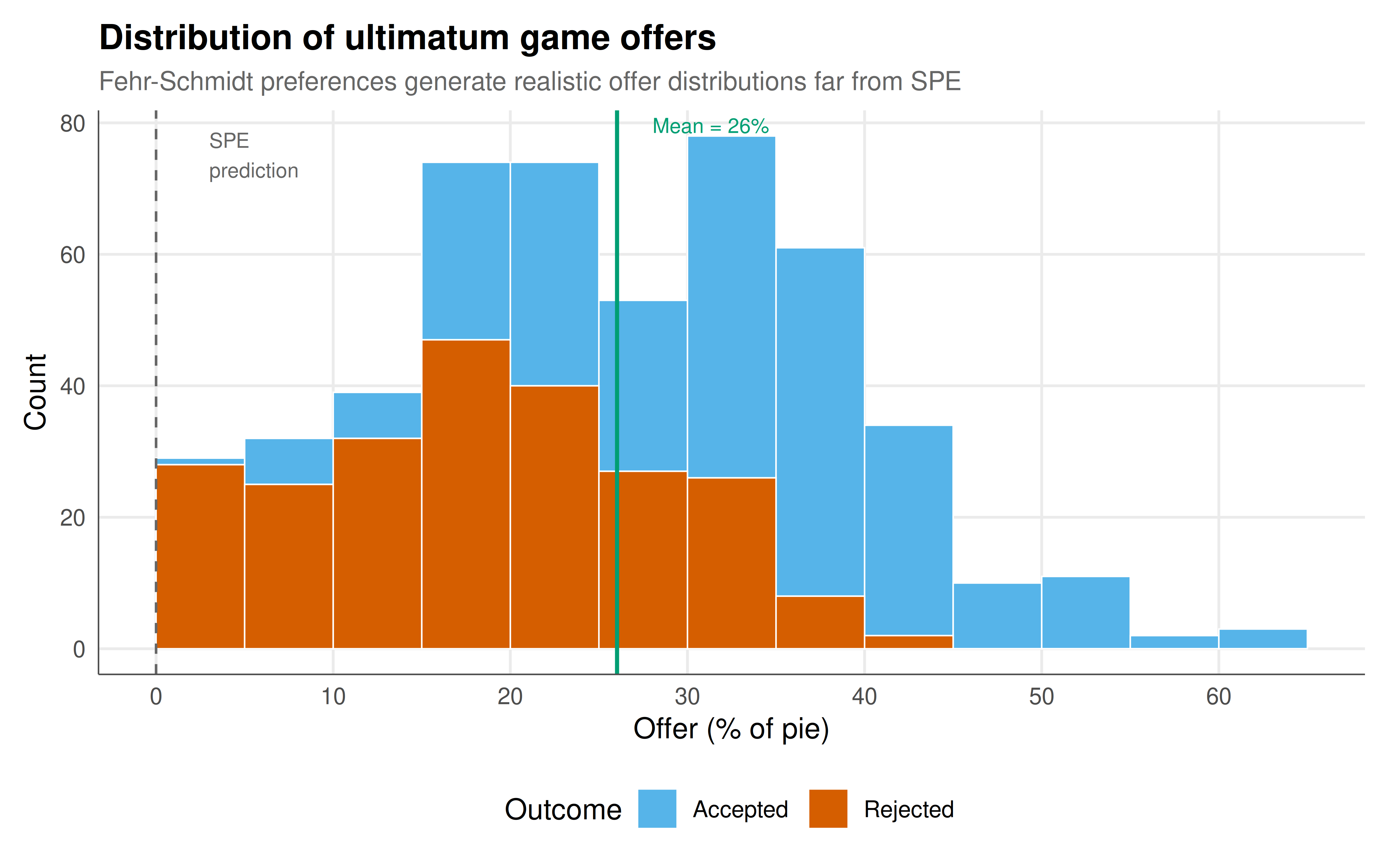
#| fig-cap: "Figure 1. Distribution of ultimatum game offers from a simulated experiment with Fehr-Schmidt preferences (N=500 proposer-responder pairs). The histogram shows offers as percentage of the pie, with bars coloured by acceptance (blue) or rejection (orange). The dashed vertical line marks the subgame-perfect prediction (offer approaching 0%), while the solid vertical line shows the mean offer around 35%. The modal bin is 30-40%, consistent with experimental evidence from cross-cultural studies. Low offers (below 20%) face high rejection rates, making them unprofitable despite keeping more of the pie. Okabe-Ito palette."
#| dev: [png, pdf]
#| fig-width: 8
#| fig-height: 5
#| dpi: 300
ggplot(exp_data, aes(x = offer_pct, fill = rejected)) +
  geom_histogram(binwidth = 5, boundary = 0, color = "white", linewidth = 0.3) +
  geom_vline(xintercept = 0, linetype = "dashed", color = "grey40", linewidth = 0.5) +
  geom_vline(xintercept = mean(offers) * 100, linetype = "solid",
             color = okabe_ito[3], linewidth = 0.8) +
  annotate("text", x = 3, y = Inf, label = "SPE\nprediction",
           vjust = 1.5, hjust = 0, size = 3, color = "grey40") +
  annotate("text", x = mean(offers)*100 + 2, y = Inf,
           label = paste0("Mean = ", round(mean(offers)*100, 1), "%"),
           vjust = 1.5, hjust = 0, size = 3, color = okabe_ito[3]) +
  scale_fill_manual(values = c("FALSE" = okabe_ito[2], "TRUE" = okabe_ito[6]),
                    name = "Outcome", labels = c("Accepted", "Rejected")) +
  labs(title = "Distribution of ultimatum game offers",
       subtitle = "Fehr-Schmidt preferences generate realistic offer distributions far from SPE",
       x = "Offer (% of pie)", y = "Count") +
  scale_x_continuous(breaks = seq(0, 100, 10)) +
  theme_publication()
```
## Interactive figure
```{r}
#| label: fig-rejection-interactive
# Rejection probability as function of offer, by preference type
offer_grid <- seq(0, 0.5, 0.01)
alpha_types <- c(0.5, 1, 2, 4)
rej_curves <- lapply(alpha_types, function(a) {
  threshold <- responder_threshold(a)
  # Smooth rejection probability with noise
  rej_prob <- pnorm(threshold - offer_grid, sd = 0.05)
  tibble(offer = offer_grid * 100, rej_prob = rej_prob,
         type = paste0("α = ", a, " (thr = ", round(threshold*100, 1), "%)"),
         text = paste0("Offer: ", round(offer_grid*100, 0), "%",
                       "\nα = ", a,
                       "\nP(reject) = ", round(rej_prob*100, 1), "%",
                       "\nThreshold: ", round(threshold*100, 1), "%"))
}) |> bind_rows()

p_rej <- ggplot(rej_curves, aes(x = offer, y = rej_prob, color = type, text = text)) +
  geom_line(linewidth = 0.9) +
  scale_color_manual(values = okabe_ito[c(1, 5, 6, 3)], name = "Inequality aversion") +
  scale_y_continuous(labels = scales::percent_format()) +
  labs(title = "Rejection probability by offer size and inequality aversion",
       subtitle = "Higher α shifts the rejection threshold rightward",
       x = "Offer (% of pie)", y = "P(reject)") +
  theme_publication()

ggplotly(p_rej, tooltip = "text") |>
  config(displaylogo = FALSE, modeBarButtonsToRemove = c("select2d", "lasso2d"))
```
## Interpretation
The ultimatum game results demonstrate one of the most robust failures of classical game theory's predictions. The subgame-perfect equilibrium — offer almost nothing, accept anything positive — assumes that players care only about their own material payoff. But experimental evidence consistently shows that proposers offer 30-50% of the pie and responders reject offers below 20% roughly half the time. This pattern holds across dozens of countries, with stakes ranging from a few dollars to several months' wages, and in both one-shot and repeated settings. Our simulation with Fehr-Schmidt preferences reproduces these stylised facts, showing that inequality aversion alone is sufficient to generate realistic offer distributions.
The Fehr-Schmidt model provides an elegant resolution: if responders experience disutility from disadvantageous inequality (being given less than half), they may rationally reject low offers because the disutility of inequality exceeds the material gain. The rejection threshold $\alpha_R / (1 + 2\alpha_R)$ increases with the envy parameter, ranging from 0% (purely selfish, $\alpha = 0$) to approaching 50% (extremely inequality-averse, $\alpha \to \infty$). Proposers who anticipate this threshold — and who may themselves feel guilt from advantageous inequality — optimally offer more than the minimum. The population heterogeneity in fairness preferences generates the observed dispersion in offers: some proposers are strategic (offering the minimum acceptable amount) while others are genuinely fair-minded (offering equal splits regardless of the responder's type).
The stake-size analysis reveals a subtle pattern: as stakes increase, mean offers decrease slightly but do not converge to the SPE prediction. This matches experimental findings — even with three months' salary at stake (as in Cameroon experiments), offers remain around 30-40%. The reduction in variance at high stakes is consistent with proposers deliberating more carefully when more money is on the table, but the persistence of substantial offers suggests that fairness preferences are not simply errors or inattention that disappear with sufficient incentives. This is important evidence against the "income effect" critique of ultimatum game results.
The cross-cultural variation in ultimatum game behaviour provides further evidence for the social-preference interpretation. Experiments in small-scale societies by Henrich et al. (2001) found substantial variation: the Machiguenga in Peru offered only 26% on average (with few rejections), while the Lamalera whale hunters of Indonesia offered 57%. These differences correlate with the degree of market integration and cooperative norms in each society, suggesting that fairness preferences are culturally transmitted and context-dependent. The Fehr-Schmidt model can accommodate this variation through different population distributions of $\alpha$ and $\beta$ parameters, making it a flexible framework for cross-cultural comparison.
## Extensions & related tutorials
- [Fehr-Schmidt inequality aversion](../../behavioral-gt/social-preferences-fehr-schmidt/index.qmd) — the utility model used here in full detail.
- [Subgame-perfect equilibrium](../../foundations/extensive-form-subgame-perfection/index.qmd) — the classical prediction that experiments reject.
- [Quantal response equilibrium](../../behavioral-gt/quantal-response-equilibrium/) — alternative approach using decision noise.
- [Prospect theory and reference dependence](../../behavioral-economics/prospect-theory-reference-dependence/) — another departure from expected utility.
- [Beauty contest experiments](../beauty-contest-guessing/index.qmd) — another classic experimental game.
## References
::: {#refs}
:::