Reading TIVITA recordings with tivis.r

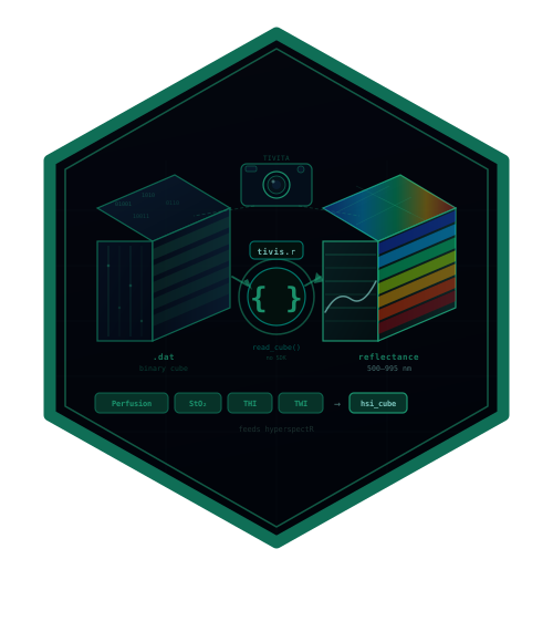
The Diaspective Vision TIVITA Suite writes each capture as a directory containing a binary *_SpecCube.dat cube, a *_meta.log acquisition record, and a set of PNG parameter maps the Suite computed itself. tivis.r reads all three. It needs no vendor SDK and contains no compiled code, which is the main practical difference from its Cubert counterpart, cuvis.r.

Everything below runs against a small example recording bundled with the package, so it works without access to clinical data.

f <- tivis_example_file()
basename(f)
#> [1] "example_SpecCube.dat"

Inspecting before reading

A full TIVITA cube is roughly 123 MB. When surveying an archive you rarely want the samples, so read the header alone — it is a 12-byte read regardless of file size.

tivis_read_header(f)
#> $width
#> [1] 16
#> 
#> $height
#> [1] 12
#> 
#> $bands
#> [1] 8
#> 
#> $n_values
#> [1] 1536
#> 
#> $file_size
#> [1] 6156

The header carries width, height and bands. Note the ordering: the header is (width, height, bands), but the array you get back is (rows, cols, bands) — height first — to match the convention used by hyperspectR::hsi_cube().

Reading a cube

cube <- tivis_read_cube(f)
dim(cube)
#> [1] 12 16  8
range(attr(cube, "wavelengths"))
#> [1] 500 535

The wavelength axis is attached as an attribute. A native TIVITA recording covers 500–995 nm in 5 nm steps across 100 bands.

head(tivis_get_wavelengths(100L))
#> [1] 500 505 510 515 520 525

Reading a subset of bands is often enough, for instance when building an RGB composite:

rgb_bands <- tivis_read_cube(f, bands = c(1L, 3L, 5L))
dim(rgb_bands)
#> [1] 12 16  3
attr(rgb_bands, "wavelengths")
#> [1] 500 510 520

Acquisition metadata

The Suite writes an INI-style log with German section names, latin1 encoding and comma decimal separators. All three are handled, and values are coerced to numerics and logicals where that is unambiguous.

log_file <- system.file("extdata", "example_meta.log", package = "tivis.r")
meta <- tivis_get_metadata(log_file)
str(meta, max.level = 2)
#> List of 4
#>  $ Camera             :List of 5
#>   ..$ CamID         : chr "0000-00000"
#>   ..$ Exposure      : num 90
#>   ..$ analoger Gain : num 8
#>   ..$ digitaler Gain: num 32
#>   ..$ Speed         : num 950
#>  $ SW                 :List of 2
#>   ..$ Name   : chr "TIVITA® Suite"
#>   ..$ Version: chr "1.6.0.1"
#>  $ Fremdlichterkennung:List of 3
#>   ..$ Fremdlicht erkannt?: logi FALSE
#>   ..$ PixelmitFremdlicht : num 0
#>   ..$ Intensity Grenzwert: num 7
#>  $ Aufnahme           :List of 1
#>   ..$ Aufnahmemodus: chr "Reflektanz"

Note that Intensity Grenzwert, written as 7,000000, comes back as the number 7 rather than a string, while text that merely contains a comma is left alone.

meta$Fremdlichterkennung$`Intensity Grenzwert`
#> [1] 7

Whole recordings and archives

tivis_measurement() bundles the cube with everything stored beside it:

m <- tivis_measurement(f)
names(m)
#> [1] "cube"        "wavelengths" "metadata"    "references"  "timestamp"  
#> [6] "path"
dim(m$cube)
#> [1] 12 16  8

For a real archive, tivis_list_measurements() walks the tree and returns one row per recording, reading only headers:

ms <- tivis_list_measurements("/archive/tivita")
nrow(ms)
unique(paste(ms$width, ms$height, ms$bands))

A note on the format

TIVITA does not publish a specification. The layout implemented here was determined empirically and then validated against the Suite’s own _RGB-Image.png exports: correlating each band of a real recording against the greyscale reference peaks at band 12, i.e. 555 nm, which is where human photopic luminous efficiency peaks. Competing hypotheses — band-sequential storage, transposed spatial axes — score near zero.

This matters because the failure mode is silent. array() recycles without complaint, so a reader with the wrong dimensions or sample type still returns a full-size cube; it is simply noise. tivis_read_header() therefore checks the file size against the header and refuses to guess.

Where this fits

tivis.r is a format reader, deliberately narrow. Cube construction, preprocessing and tissue indices live in hyperspectR; publication-grade rendering lives in hyperspectaculR.