
Statistical Analysis of Cell-Based Assays
Source:vignettes/statistical-analysis.Rmd
statistical-analysis.RmdWhy the level of aggregation matters
In a microscopy-based cell assay each treatment condition is measured across several wells, and each well holds many cells. Cells within a well are not independent: they share staining, focus and exposure. Treating every cell as an independent replicate inflates the sample size and, with it, the confidence of the answer.
cellreportR supports both resolutions and asks you to say which one you mean:
- Cell-level tests treat each cell as a data point. Use them for distributional questions — is there a subpopulation shift, does a marker separate two conditions.
- Replicate-level tests aggregate cells to one number per well and test wells. Use them for the primary inference about whether a compound has an effect.
Run both, report the effect size with its interval at the replicate level, and let the difference between the two be visible rather than assumed.
A worked example
exp <- cr_example_experiment(seed = 2, n_cells_per_well = 60)

res <- cr_test(exp,
               channel   = "marker_1",
               treatment = "CompoundA_high",
               control   = "Untreated",
               test      = "mann_whitney",
               level     = "both")

res$cell_level
#> # A tibble: 1 × 8
#>   level test         statistic p_value   n_x   n_y median_x median_y
#>   <chr> <chr>            <dbl>   <dbl> <int> <int>    <dbl>    <dbl>
#> 1 cell  mann_whitney    904417       0   969   941    4143.     553.
res$rep_level
#> # A tibble: 1 × 8
#>   level     test         statistic    p_value   n_x   n_y median_x median_y
#>   <chr>     <chr>            <dbl>      <dbl> <int> <int>    <dbl>    <dbl>
#> 1 replicate mann_whitney       256 0.00000154    16    16    4175.     550.
Same data, same contrast. The cell-level test is run on nearly two thousand observations and the replicate-level test on thirty-two, and the p-values differ by orders of magnitude. The extra cells did not add independent information; they only made the arithmetic behave as though they had.
cr_test() also returns effect sizes, computed on the
cells:
res$effect_sizes
#> # A tibble: 4 × 5
#>   method        estimate ci_low ci_high magnitude
#>   <chr>            <dbl>  <dbl>   <dbl> <chr>
#> 1 cohens_d         2.22   2.10    2.33  large
#> 2 hedges_g         2.22   2.10    2.33  large
#> 3 cliffs_delta     0.984  0.976   0.989 large
#> 4 rank_biserial    0.984  0.976   0.989 large
Those intervals are cell-level intervals whatever level
was asked for, so they are narrow for exactly the reason the cell-level
p-value is small. For an interval that respects the unit of replication,
use cr_effect_grid() with unit set —
vignette("end-to-end") puts the two side by side and
measures the gap.
Effect size interpretation
cr_effect_size() computes Cohen’s d, Hedges’
g, Cliff’s delta, rank-biserial correlation and Glass’s delta,
each with a confidence interval. The verbal magnitude attached to an
estimate uses the conventional benchmarks:
| Magnitude | Cohen’s d, Hedges’ g, Glass’s delta | Cliff’s delta, rank-biserial |
|---|---|---|
| negligible | |est| < 0.2 | |est| < 0.147 |
| small | 0.2 – 0.5 | 0.147 – 0.33 |
| medium | 0.5 – 0.8 | 0.33 – 0.474 |
| large | ≥ 0.8 | ≥ 0.474 |
set.seed(1)
cr_effect_size(rnorm(100, 1), rnorm(100, 0))
#> # A tibble: 5 × 5
#>   method        estimate ci_low ci_high magnitude
#>   <chr>            <dbl>  <dbl>   <dbl> <chr>
#> 1 cohens_d         1.23   0.930   1.54  large
#> 2 hedges_g         1.23   0.927   1.53  large
#> 3 cliffs_delta     0.616  0.481   0.723 large
#> 4 rank_biserial    0.616  0.481   0.723 large
#> 5 glass_delta      1.20   0.872   1.52  large
Bootstrap intervals are available where the analytic ones do not apply:
set.seed(1)
cr_effect_size(rnorm(60, 0.8), rnorm(60, 0),
               method = "cliffs_delta",
               ci_method = "bootstrap", n_boot = 200, seed = 1)
#> # A tibble: 1 × 5
#>   method       estimate ci_low ci_high magnitude
#>   <chr>           <dbl>  <dbl>   <dbl> <chr>
#> 1 cliffs_delta    0.495  0.356   0.649 large
ROC and AUC for discriminability
“Does this marker tell a treated cell from a control cell?” is a different question from “did the group means move”, and it has a different answer. Fit a univariate logistic regression and read the area under the curve:
logit <- cr_logistic(exp, "marker_1", "CompoundA_high", "Untreated")
cr_auc(logit)
#> # A tibble: 1 × 4
#>     auc ci_low ci_high method
#>   <dbl>  <dbl>   <dbl> <chr>
#> 1 0.992  0.989   0.995 delong
cr_plot_roc(logit)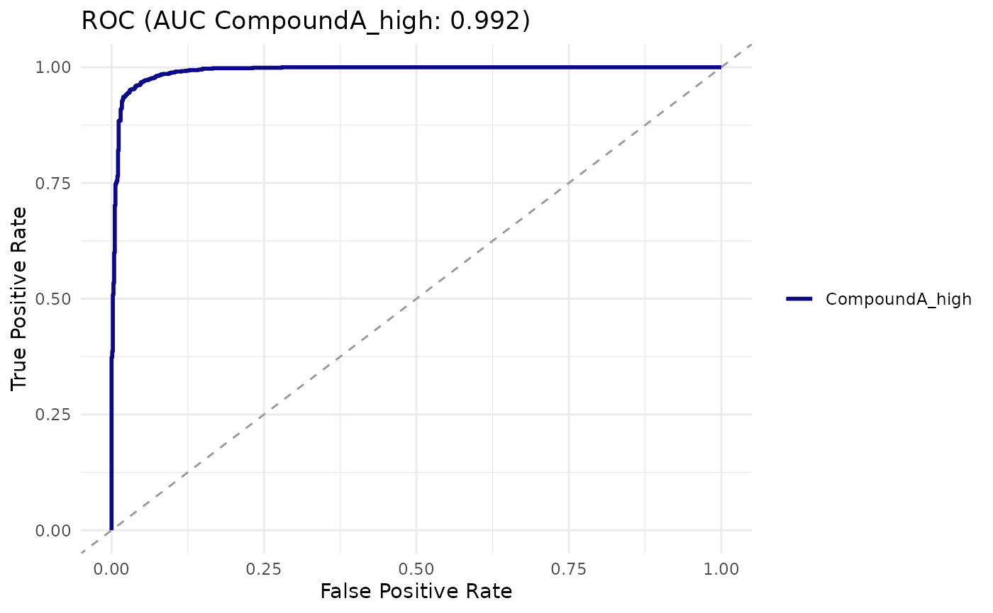
cr_confusion_matrix(logit, threshold = 0.5)
#> # A tibble: 1 × 10
#>   threshold sensitivity specificity   ppv   npv accuracy    tp    tn    fp    fn
#>       <dbl>       <dbl>       <dbl> <dbl> <dbl>    <dbl> <int> <int> <int> <int>
#> 1       0.5       0.951       0.967 0.967 0.951    0.959   922   910    31    47
Multiple testing
cr_test_all() runs every treatment level against the
control and reports the adjustments alongside the
unadjusted p-value, never in place of it:
all_res <- cr_test_all(exp, "marker_1", "Untreated", level = "replicate")
attr(all_res, "summary")[, c("treatment", "log2_fc", "p_value",
                             "p_bonferroni", "p_BH", "interpretation")]
#> # A tibble: 5 × 6
#>   treatment      log2_fc    p_value p_bonferroni       p_BH interpretation
#>   <chr>            <dbl>      <dbl>        <dbl>      <dbl> <chr>
#> 1 PosControl       3.10  0.00000154   0.00000772 0.00000386 strong
#> 2 CompoundA_low    0.916 0.0000312    0.000156   0.0000520  strong
#> 3 CompoundA_high   2.92  0.00000154   0.00000772 0.00000386 strong
#> 4 CompoundB        0.314 0.109        0.546      0.109      no evidence
#> 5 CompoundC        0.578 0.0000433    0.000216   0.0000541  moderate
The interpretation column combines the adjusted p-value
with the effect size: a contrast is "weak",
"moderate" or "strong" only when
p_adj < 0.05, and "no evidence"
otherwise.
Power and sample size
cr_power_analysis() simulates the two-sample t-test that
a replicate-level analysis actually runs: n_replicates
replicate means per arm, each the average of
n_cells_per_rep draws, tested against each other.
cr_power_analysis(effect_size     = 0.3,
                  n_replicates    = 4,
                  n_cells_per_rep = 20,
                  n_sim           = 200,
                  seed            = 1)
#> # A tibble: 1 × 5
#>   effect_size n_replicates n_cells_per_rep alpha power
#>         <dbl>        <dbl>           <dbl> <dbl> <dbl>
#> 1         0.3            4              20  0.05 0.355
Read the number for what the simulation models. The only source of
spread between replicate means here is the averaging itself, so power
rises steeply with n_cells_per_rep. Real units also differ
from one another for reasons that more cells cannot average away —
staining, focus, seeding density — and that component is not in this
model. The figure is therefore an upper bound: a design
that fails here will certainly fail in the laboratory, and one that
passes here may still not.
For sizing a follow-up study from effects you have actually observed
rather than from an assumed one, use cr_power_grid(), which
solves from the confidence bound nearer the null and so inherits the
between-unit variability of the data it was given — see
vignette("end-to-end").
Where this fits
-
vignette("getting-started")— the short path on one plate. -
vignette("end-to-end")— the same choice of level made across a whole screen, withcr_effect_grid()andcr_compare_levels()quantifying the gap between the two.