Week 4, Session 3 — Pearson and Spearman correlation

Course 1 — #courses

Author

R. Heller

Note

Inference labs use the five-step template: Hypothesis → Visualise → Assumptions → Conduct → Conclude.

Learning objectives

Compute Pearson and Spearman correlations with cor.test() and interpret the coefficient and its CI.
Distinguish linear association from monotonic association.
Use visualisation to diagnose situations where a correlation coefficient misleads (Anscombe, DatasauRus).

Prerequisites

Week 1, Lab 2.5.

Background

Pearson’s r measures linear association. It is the standardised covariance of two variables; it is sensitive to outliers and assumes a roughly linear, bivariate-normal relationship. Spearman’s ρ measures monotonic association. It is Pearson’s r applied to the ranks of the variables; it is robust to outliers and to non-linear monotonic transformations.

Neither coefficient captures non-linear, non-monotonic relationships well. Anscombe’s quartet and the DatasauRus dozen are the canonical demonstrations that a coefficient without a plot can lie — datasets engineered to have identical Pearson r but radically different shapes. The conclusion is not to abandon correlations but never to report one without first plotting the data.

A correlation coefficient is not a causal quantity. Two variables can be perfectly correlated without one causing the other — a lurking variable, a common cause, a coincidence of sample selection. The word “correlation” is often used loosely in the press to mean “weak causation”; in this course it means exactly what cor.test() returns.

Setup

library(tidyverse)
library(datasauRus)
set.seed(42)
theme_set(theme_minimal(base_size = 12))

1. Hypothesis

Two scenarios:

A linear relationship between two simulated variables.
A monotonic but non-linear relationship where Pearson misleads.

H0 in each case: ρ = 0. H1: ρ ≠ 0.

2. Visualise

n <- 200
x <- rnorm(n)
y_linear   <- 0.6 * x + rnorm(n, 0, 0.8)
y_monotone <- exp(x) + rnorm(n, 0, 0.5)
df <- tibble(x, y_linear, y_monotone) |>
  pivot_longer(starts_with("y_"), names_to = "type", values_to = "y")

df |>
  ggplot(aes(x, y)) +
  geom_point(alpha = 0.5) +
  facet_wrap(~ type, scales = "free") +
  geom_smooth(method = "lm", se = FALSE, colour = "firebrick", linewidth = 0.5)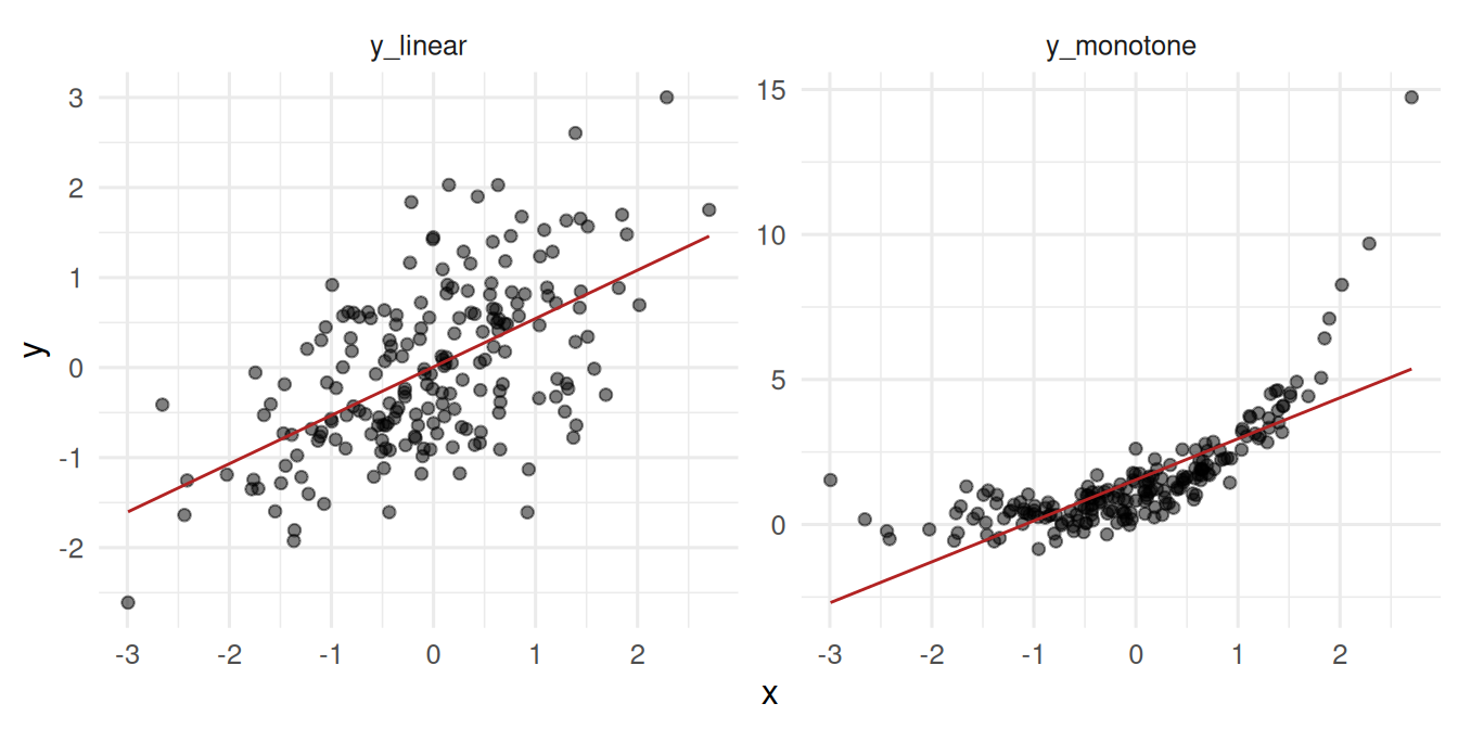

3. Assumptions

Pearson assumes linearity and roughly bivariate-normal data. Spearman assumes monotonicity. Neither handles non-monotonic relationships. For both, the observations must be independent; both are sensitive to extreme sample-size-induced significance when n is huge.

4. Conduct

p1_pearson  <- cor.test(x, y_linear,   method = "pearson")
p1_spearman <- cor.test(x, y_linear,   method = "spearman", exact = FALSE)
p2_pearson  <- cor.test(x, y_monotone, method = "pearson")
p2_spearman <- cor.test(x, y_monotone, method = "spearman", exact = FALSE)

tibble(
  relationship = c("linear", "linear", "monotone", "monotone"),
  method = c("Pearson", "Spearman", "Pearson", "Spearman"),
  r_or_rho = c(p1_pearson$estimate, p1_spearman$estimate,
               p2_pearson$estimate, p2_spearman$estimate),
  p = c(p1_pearson$p.value, p1_spearman$p.value,
        p2_pearson$p.value, p2_spearman$p.value)
)

# A tibble: 4 × 4
  relationship method   r_or_rho        p
  <chr>        <chr>       <dbl>    <dbl>
1 linear       Pearson     0.570 1.27e-18
2 linear       Spearman    0.528 8.89e-16
3 monotone     Pearson     0.762 2.90e-39
4 monotone     Spearman    0.833 7.32e-53

The monotonic non-linear relationship gives a much higher Spearman than Pearson — the rank correlation sees the perfect monotonicity.

The DatasauRus demonstration

ds_summary <- datasaurus_dozen |>
  group_by(dataset) |>
  summarise(mean_x = mean(x),
            mean_y = mean(y),
            sd_x = sd(x),
            sd_y = sd(y),
            r = cor(x, y), .groups = "drop")
head(ds_summary)

# A tibble: 6 × 6
  dataset  mean_x mean_y  sd_x  sd_y       r
  <chr>     <dbl>  <dbl> <dbl> <dbl>   <dbl>
1 away       54.3   47.8  16.8  26.9 -0.0641
2 bullseye   54.3   47.8  16.8  26.9 -0.0686
3 circle     54.3   47.8  16.8  26.9 -0.0683
4 dino       54.3   47.8  16.8  26.9 -0.0645
5 dots       54.3   47.8  16.8  26.9 -0.0603
6 h_lines    54.3   47.8  16.8  26.9 -0.0617

datasaurus_dozen |>
  ggplot(aes(x, y)) +
  geom_point(alpha = 0.4, size = 0.8) +
  facet_wrap(~ dataset) +
  labs(x = NULL, y = NULL)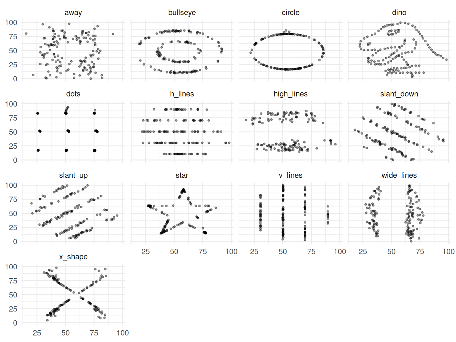

Thirteen datasets; all have mean x ≈ 54, mean y ≈ 47, SDs ≈ 17 and 26, and Pearson r ≈ −0.06. The shapes are wildly different.

5. Concluding statement

In the linear case, Pearson r = 0.57 (p = 1.3^{-18}) and Spearman ρ = 0.53; the two agreed. In the monotonic non-linear case, Pearson r = 0.76 was substantially smaller than Spearman ρ = 0.83, revealing that the association was strong but not linear. The DatasauRus dozen reproduced identical summary statistics across 13 radically different shapes, reinforcing the rule: never report a correlation without the scatter plot.

Correlation is a single number. Its honest use requires a picture alongside.

Show the DatasauRus grid large and silent for ten seconds — the visual impact makes the point that no verbal argument can.

Common pitfalls

Reporting a Pearson r on data with an obvious curvilinear shape.
Using r to compare groups with different sample sizes; small r can be “significant” at huge n.
Inferring causation from a correlation.
Computing correlations on data that include outliers without a robustness check.

Session info

sessionInfo()

R version 4.4.1 (2024-06-14)
Platform: x86_64-pc-linux-gnu
Running under: Ubuntu 24.04.4 LTS

Matrix products: default
BLAS:   /usr/lib/x86_64-linux-gnu/openblas-pthread/libblas.so.3 
LAPACK: /usr/lib/x86_64-linux-gnu/openblas-pthread/libopenblasp-r0.3.26.so;  LAPACK version 3.12.0

locale:
 [1] LC_CTYPE=C.UTF-8       LC_NUMERIC=C           LC_TIME=C.UTF-8       
 [4] LC_COLLATE=C.UTF-8     LC_MONETARY=C.UTF-8    LC_MESSAGES=C.UTF-8   
 [7] LC_PAPER=C.UTF-8       LC_NAME=C              LC_ADDRESS=C          
[10] LC_TELEPHONE=C         LC_MEASUREMENT=C.UTF-8 LC_IDENTIFICATION=C   

time zone: UTC
tzcode source: system (glibc)

attached base packages:
[1] stats     graphics  grDevices utils     datasets  methods   base     

other attached packages:
 [1] datasauRus_0.1.9 lubridate_1.9.5  forcats_1.0.1    stringr_1.6.0   
 [5] dplyr_1.2.1      purrr_1.2.2      readr_2.2.0      tidyr_1.3.2     
 [9] tibble_3.3.1     ggplot2_4.0.3    tidyverse_2.0.0 

loaded via a namespace (and not attached):
 [1] Matrix_1.7-0       gtable_0.3.6       jsonlite_2.0.0     compiler_4.4.1    
 [5] tidyselect_1.2.1   splines_4.4.1      scales_1.4.0       yaml_2.3.12       
 [9] fastmap_1.2.0      lattice_0.22-6     R6_2.6.1           labeling_0.4.3    
[13] generics_0.1.4     knitr_1.51         htmlwidgets_1.6.4  pillar_1.11.1     
[17] RColorBrewer_1.1-3 tzdb_0.5.0         rlang_1.2.0        utf8_1.2.6        
[21] stringi_1.8.7      xfun_0.57          S7_0.2.2           otel_0.2.0        
[25] timechange_0.4.0   cli_3.6.6          mgcv_1.9-1         withr_3.0.2       
[29] magrittr_2.0.5     digest_0.6.39      grid_4.4.1         hms_1.1.4         
[33] nlme_3.1-164       lifecycle_1.0.5    vctrs_0.7.3        evaluate_1.0.5    
[37] glue_1.8.1         farver_2.1.2       rmarkdown_2.31     tools_4.4.1       
[41] pkgconfig_2.0.3    htmltools_0.5.9

Learning objectives

Prerequisites

Background

Setup

1. Hypothesis

2. Visualise

3. Assumptions

4. Conduct

The DatasauRus demonstration

5. Concluding statement

Common pitfalls

Further reading

Session info

Related labs