library(tidyverse)
library(mgcv)
library(gratia)
library(broom)
set.seed(42)
theme_set(theme_minimal(base_size = 12))Week 2, Session 4 — GAMs with mgcv
Course 2 — #courses
Note
Inference labs use the five-step template: Hypothesis → Visualise → Assumptions → Conduct → Conclude.
Learning objectives
- Fit a generalised additive model with
mgcv::gam()and a single smooth term. - Read effective degrees of freedom as a data-driven measure of flexibility.
- Visualise a smooth with
gratia::draw()and report its shape in plain language.
Prerequisites
Sessions 1–2 of Week 1.
Background
Generalised additive models replace the linear term β·X in a regression with a smooth function f(X) estimated from the data. The smooth is regularised so that wiggliness is penalised; the penalty strength is chosen by restricted maximum likelihood or generalised cross-validation. The effective degrees of freedom (edf) of the smooth quantifies how much of that flexibility was used: an edf near 1 means the smooth is essentially a line; an edf of 5 means something meaningfully curved.
GAMs are particularly useful when the shape of the relationship is the scientific question. They are also useful as diagnostics for linear models, because plotting a smooth against a predictor can reveal a curve that the linear term would miss.
The mgcv package is the reference implementation. gratia is a newer graphics layer on top of mgcv that produces tidy, ggplot-based plots of smooths, partial effects, and derivatives.
Setup
1. Hypothesis
Simulate a sine-wave-plus-noise relationship and ask whether a GAM recovers it while a linear model misses it.
2. Visualise
n <- 300
x <- runif(n, 0, 4 * pi)
y <- sin(x) + rnorm(n, 0, 0.4)
dat <- tibble(x, y)

ggplot(dat, aes(x, y)) +
  geom_point(alpha = 0.5, colour = "grey30") +
  labs(x = "x", y = "y")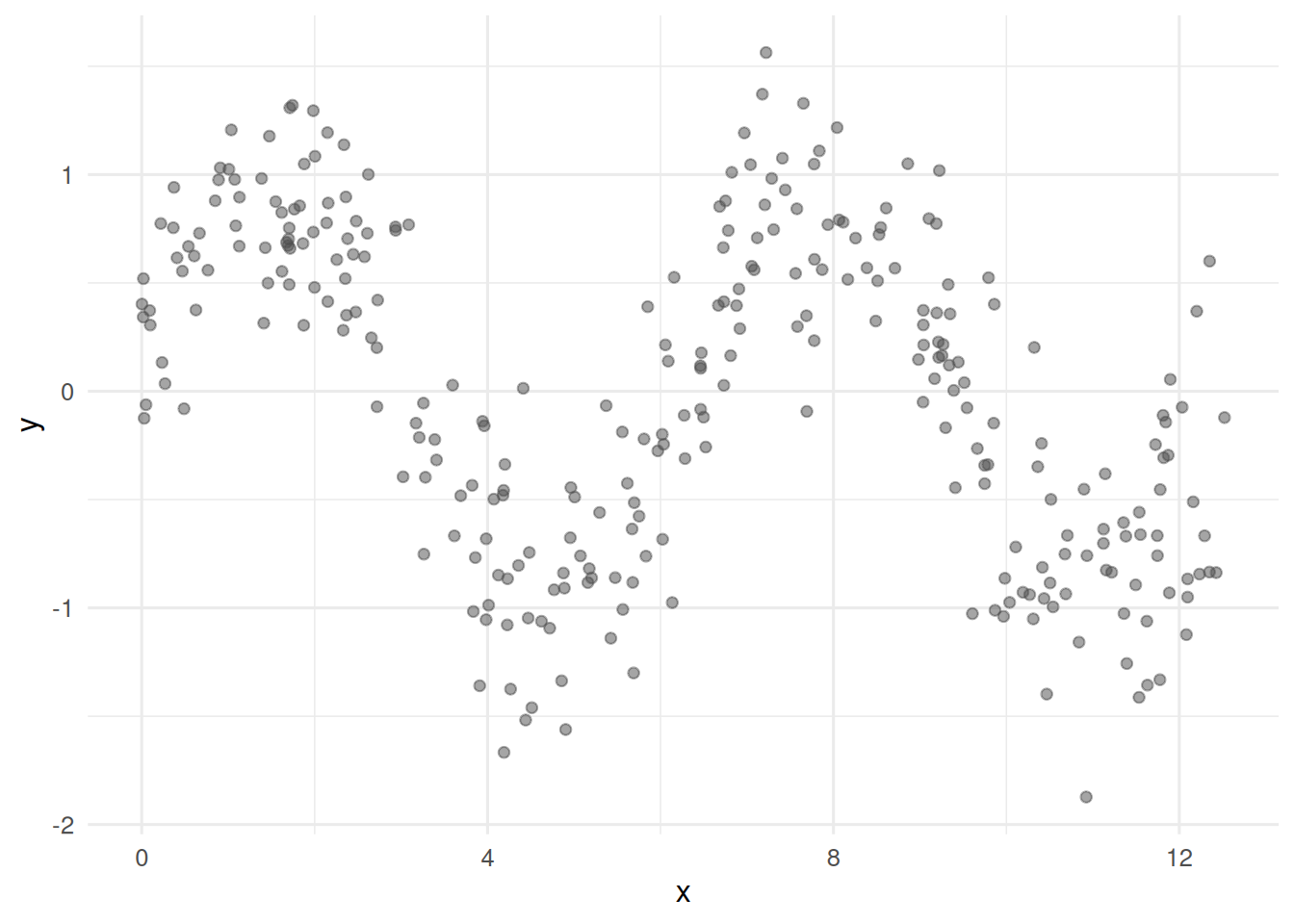
3. Assumptions
GAMs assume independent observations and a correctly specified response distribution. The smooth flexibility is chosen automatically; the user chooses the basis and, if relevant, the upper limit on flexibility via k.
fit_lm  <- lm(y ~ x, data = dat)
fit_gam <- gam(y ~ s(x, bs = "cr", k = 20), data = dat, method = "REML")

plot(fit_gam, residuals = TRUE, pch = 1, shade = TRUE)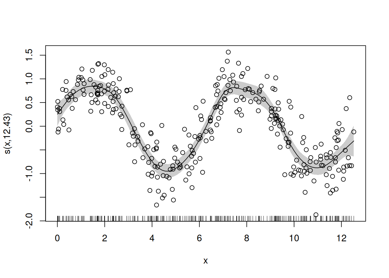
gam.check(fit_gam)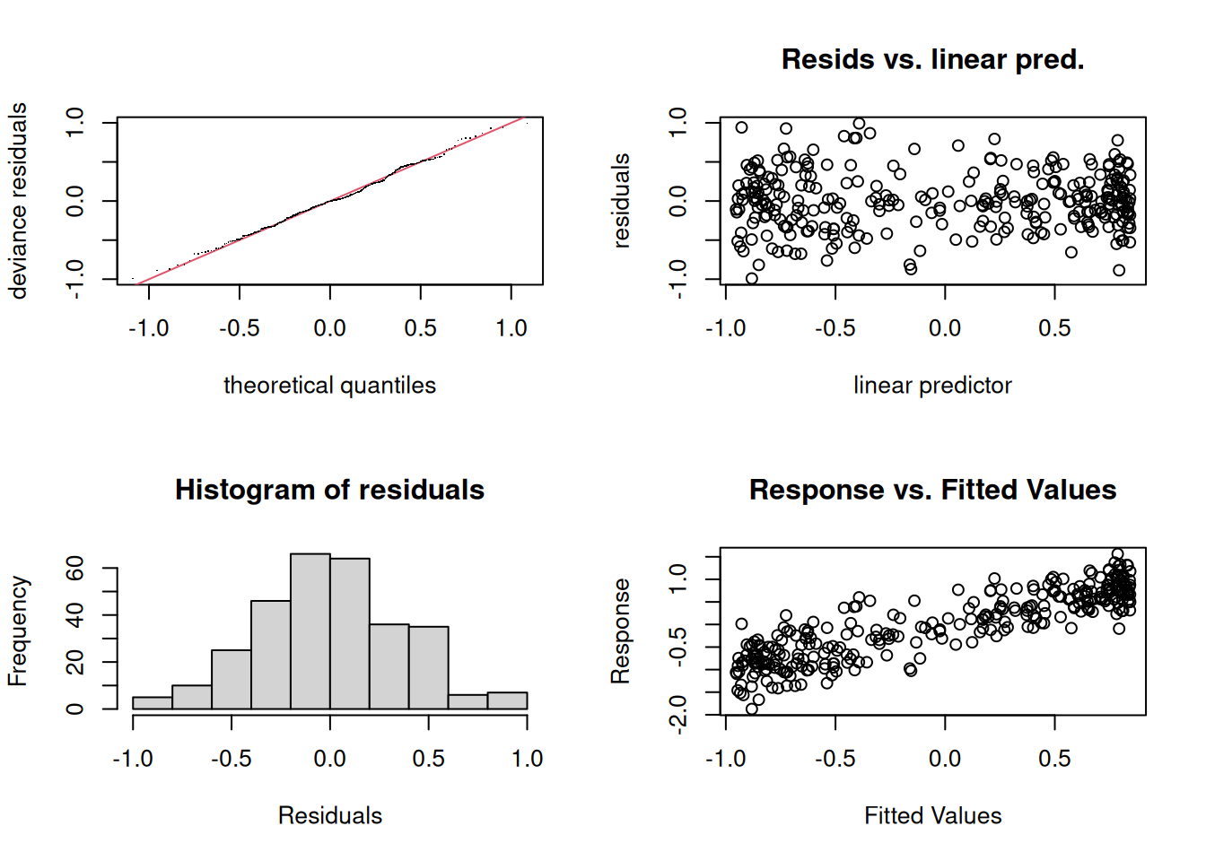
Method: REML   Optimizer: outer newton
full convergence after 4 iterations.
Gradient range [-5.838318e-05,1.726219e-06]
(score 150.8396 & scale 0.1374259).
Hessian positive definite, eigenvalue range [4.979807,149.2267].
Model rank =  20 / 20

Basis dimension (k) checking results. Low p-value (k-index<1) may
indicate that k is too low, especially if edf is close to k'.

       k'  edf k-index p-value
s(x) 19.0 12.4    1.11    0.99
gam.check reports k-index and effective df — an indication of whether k is large enough.
4. Conduct
summary(fit_gam)
Family: gaussian
Link function: identity

Formula:
y ~ s(x, bs = "cr", k = 20)

Parametric coefficients:
             Estimate Std. Error t value Pr(>|t|)
(Intercept) -0.002187   0.021403  -0.102    0.919

Approximate significance of smooth terms:
       edf Ref.df     F p-value
s(x) 12.43   14.8 62.12  <2e-16 ***
---
Signif. codes:  0 '***' 0.001 '**' 0.01 '*' 0.05 '.' 0.1 ' ' 1

R-sq.(adj) =  0.755   Deviance explained = 76.5%
-REML = 150.84 Scale est. = 0.13743 n = 300AIC(fit_lm, fit_gam) df AIC
fit_lm 3.00000 631.7192
fit_gam 14.69402 271.6137draw(fit_gam)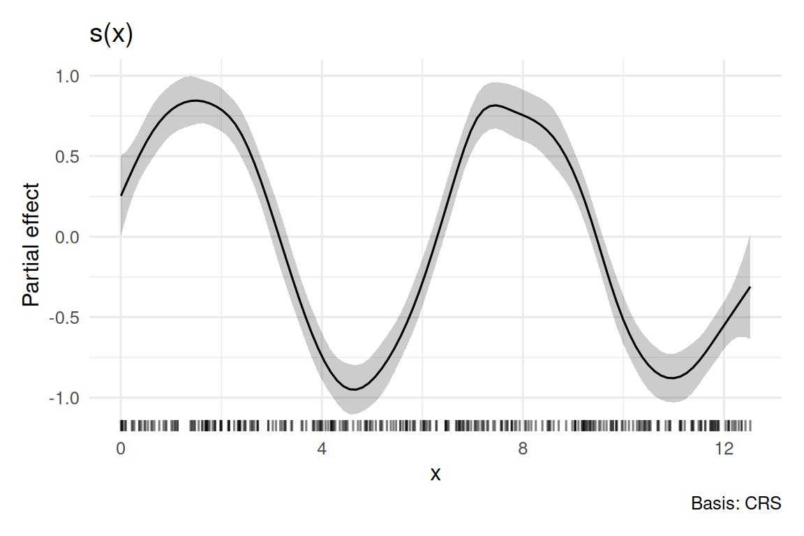
5. Concluding statement
A GAM with a single smooth of x captured the non-linear relationship (edf = 12.4; approximate p < 0.001). A linear model gave a near-zero slope because the underlying function is a full sine wave. The GAM is preferred when the shape, not a scalar slope, is the scientific object.
Explain that a large edf is not a problem; the penalty prevents the smooth from interpolating noise. The p-value reported for a smooth is approximate.
Common pitfalls
- Setting
ktoo small and constraining the smooth. - Comparing GAMs with AIC as if it were a likelihood-ratio test.
- Reporting only the smooth without showing its plot.
Further reading
- Wood SN. Generalized Additive Models: An Introduction with R.
- Pedersen EJ et al. (2019), Hierarchical generalized additive models.
- Simpson GL. gratia package vignette.
Session info
sessionInfo()R version 4.5.2 (2025-10-31 ucrt)
Platform: x86_64-w64-mingw32/x64
Running under: Windows 11 x64 (build 26200)
Matrix products: default
LAPACK version 3.12.1
locale:
[1] LC_COLLATE=English_Germany.utf8 LC_CTYPE=English_Germany.utf8
[3] LC_MONETARY=English_Germany.utf8 LC_NUMERIC=C
[5] LC_TIME=English_Germany.utf8
time zone: Europe/Berlin
tzcode source: internal
attached base packages:
[1] stats graphics grDevices utils datasets methods base
other attached packages:
[1] broom_1.0.12 gratia_0.11.2 mgcv_1.9-4 nlme_3.1-169
[5] lubridate_1.9.5 forcats_1.0.1 stringr_1.6.0 dplyr_1.2.1
[9] purrr_1.2.2 readr_2.2.0 tidyr_1.3.2 tibble_3.3.1
[13] ggplot2_4.0.3 tidyverse_2.0.0
loaded via a namespace (and not attached):
[1] generics_0.1.4 stringi_1.8.7 lattice_0.22-9 hms_1.1.4
[5] digest_0.6.39 magrittr_2.0.4 evaluate_1.0.5 grid_4.5.2
[9] timechange_0.4.0 RColorBrewer_1.1-3 fastmap_1.2.0 jsonlite_2.0.0
[13] Matrix_1.7-5 backports_1.5.1 ggokabeito_0.1.0 scales_1.4.0
[17] cli_3.6.6 rlang_1.2.0 splines_4.5.2 withr_3.0.2
[21] yaml_2.3.12 otel_0.2.0 tools_4.5.2 tzdb_0.5.0
[25] nanonext_1.9.0 vctrs_0.7.3 R6_2.6.1 lifecycle_1.0.5
[29] tweedie_3.0.19 htmlwidgets_1.6.4 pkgconfig_2.0.3 pillar_1.11.1
[33] gtable_0.3.6 glue_1.8.1 Rcpp_1.1.1-1.1 statmod_1.5.1
[37] xfun_0.57 tidyselect_1.2.1 knitr_1.51 farver_2.1.2
[41] patchwork_1.3.2 htmltools_0.5.9 mirai_2.6.1 labeling_0.4.3
[45] rmarkdown_2.31 compiler_4.5.2 S7_0.2.2 mvnfast_0.2.8