library(tidyverse)
library(broom)
set.seed(42)
theme_set(theme_minimal(base_size = 12))Week 4, Session 1 — Dichotomisation, change scores, regression to the mean
Course 2 — #courses
Note
Inference labs use the five-step template: Hypothesis → Visualise → Assumptions → Conduct → Conclude.
Learning objectives
- Quantify the power loss of a median split on a continuous predictor.
- Demonstrate regression to the mean in a simulated pre-post design.
- Distinguish apparent improvement due to RTM from a true treatment effect.
Prerequisites
Basic regression; ANCOVA from Week 3 Session 2.
Background
Dichotomising a continuous predictor — high vs low — loses information in proportion to the variability thrown away. A well-known rule of thumb is that the median split reduces power in a comparison equivalent to throwing away roughly a third of the sample. The only time a dichotomy is defensible is when the clinical decision it feeds into is itself binary, and even then the continuous underlying variable should enter the analysis.
Regression to the mean is a statistical fact about correlated pairs of measurements: participants who score unusually high on a first measurement will, on average, score less extremely on a second measurement of the same quantity, even with no intervention. In a pre-post study this produces apparent improvement in the high baseline group and apparent worsening in the low baseline group. ANCOVA handles this automatically; a simple comparison of pre and post in the extreme group does not.
RTM is not the same as measurement error, but measurement error is one source of RTM. Any non-perfect correlation between measurements produces it. This is why baseline stratification by a continuous variable must be prespecified — selecting on a single noisy baseline guarantees RTM.
Setup
1. Hypothesis
Two simulations:
- A continuous predictor truly associated with a continuous outcome; compare the p-value when treated as continuous vs median-split.
- A pre-post dataset with no intervention; show apparent improvement in the high-baseline group.
2. Visualise
n <- 200
x <- rnorm(n)
y <- 0.3 * x + rnorm(n, 0, 1)
dat1 <- tibble(x, y, x_bin = factor(ifelse(x > median(x), "high", "low")))

ggplot(dat1, aes(x, y)) +
  geom_point(alpha = 0.5) +
  geom_smooth(method = "lm", colour = "steelblue") +
  labs(x = "x (continuous)", y = "y")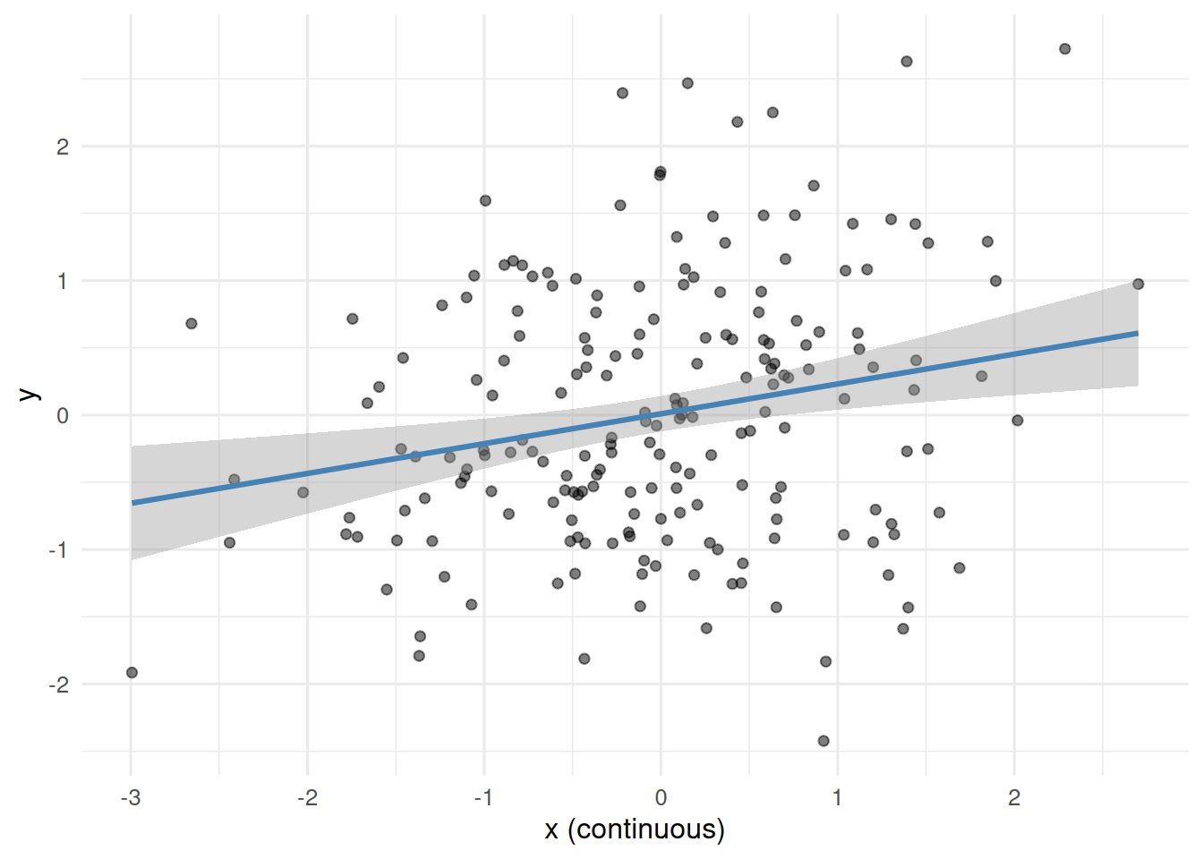
3. Assumptions
Independence, approximate normality; standard regression assumptions.
4. Conduct
Power loss from dichotomisation:
tidy(lm(y ~ x, data = dat1)) # continuous# A tibble: 2 × 5
term estimate std.error statistic p.value
<chr> <dbl> <dbl> <dbl> <dbl>
1 (Intercept) 0.00914 0.0669 0.136 0.892
2 x 0.222 0.0688 3.22 0.00148tidy(lm(y ~ x_bin, data = dat1)) # median split# A tibble: 2 × 5
term estimate std.error statistic p.value
<chr> <dbl> <dbl> <dbl> <dbl>
1 (Intercept) 0.191 0.0952 2.01 0.0463
2 x_binlow -0.376 0.135 -2.79 0.00577The p-value for x_bin should be larger than for x; the standard error is larger and the estimate is attenuated.
Regression to the mean:
n2 <- 1000
pre  <- rnorm(n2, 100, 15)
post <- 0.7 * (pre - 100) + 100 + rnorm(n2, 0, 11)
dat2 <- tibble(pre, post) |>
  mutate(high_baseline = pre > quantile(pre, 0.8))

dat2 |>
  group_by(high_baseline) |>
  summarise(pre_mean = mean(pre), post_mean = mean(post),
            change = mean(post - pre))
# A tibble: 2 × 4
high_baseline pre_mean post_mean change
<lgl> <dbl> <dbl> <dbl>
1 FALSE 94.2 96.2 2.00
2 TRUE 120. 114. -6.30The “high baseline” group shows a large negative mean change; the rest of the sample shows a small positive change. No intervention occurred.
ggplot(dat2, aes(pre, post)) +
  geom_point(alpha = 0.3) +
  geom_abline(slope = 1, intercept = 0, linetype = 2, colour = "grey50") +
  geom_smooth(method = "lm", colour = "firebrick") +
  labs(x = "Baseline", y = "Follow-up")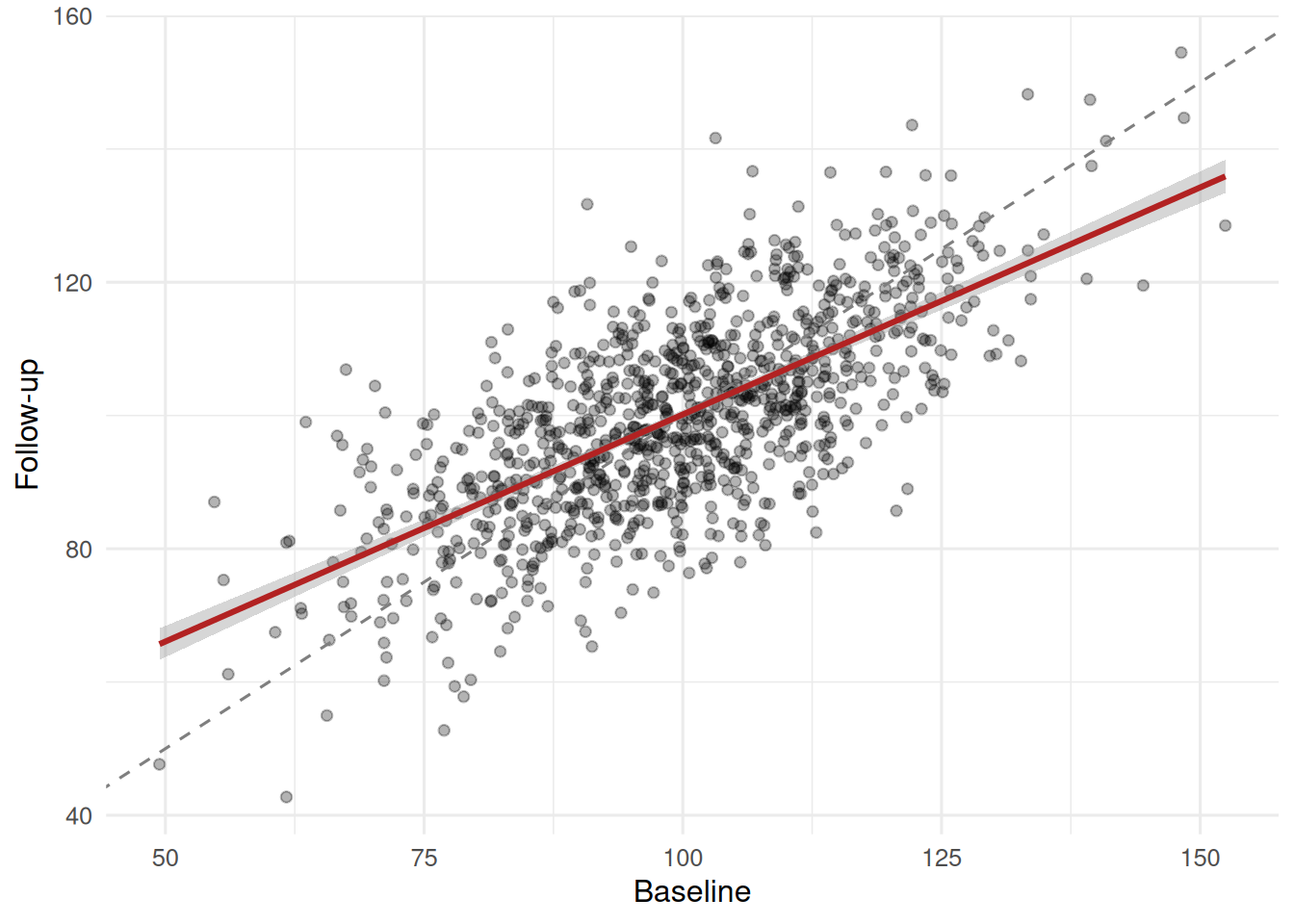
The fitted line is flatter than the identity line; that flattening is RTM.
5. Concluding statement
Dichotomising the continuous predictor inflated its p-value from 0.0015 to 0.0058 and widened its standard error. In the pre-post simulation with no intervention, the top-baseline quintile showed a mean decline of -6.3 units, entirely attributable to regression to the mean.
If time permits, loop the power simulation at different effect sizes to make the power loss visceral.
Common pitfalls
- Dichotomising to avoid thinking about the slope.
- Comparing pre-post within a high-baseline subgroup and calling the decline an effect.
- Using a paired t-test on change in a selected subgroup.
Further reading
- MacCallum RC et al. (2002), On the practice of dichotomization…
- Altman DG, Royston P (2006), The cost of dichotomising continuous…
- Senn S (2011), Francis Galton and regression to the mean.
Session info
sessionInfo()R version 4.5.2 (2025-10-31 ucrt)
Platform: x86_64-w64-mingw32/x64
Running under: Windows 11 x64 (build 26200)
Matrix products: default
LAPACK version 3.12.1
locale:
[1] LC_COLLATE=English_Germany.utf8 LC_CTYPE=English_Germany.utf8
[3] LC_MONETARY=English_Germany.utf8 LC_NUMERIC=C
[5] LC_TIME=English_Germany.utf8
time zone: Europe/Berlin
tzcode source: internal
attached base packages:
[1] stats graphics grDevices utils datasets methods base
other attached packages:
[1] broom_1.0.12 lubridate_1.9.5 forcats_1.0.1 stringr_1.6.0
[5] dplyr_1.2.1 purrr_1.2.2 readr_2.2.0 tidyr_1.3.2
[9] tibble_3.3.1 ggplot2_4.0.3 tidyverse_2.0.0
loaded via a namespace (and not attached):
[1] Matrix_1.7-5 gtable_0.3.6 jsonlite_2.0.0 compiler_4.5.2
[5] tidyselect_1.2.1 splines_4.5.2 scales_1.4.0 yaml_2.3.12
[9] fastmap_1.2.0 lattice_0.22-9 R6_2.6.1 labeling_0.4.3
[13] generics_0.1.4 knitr_1.51 backports_1.5.1 htmlwidgets_1.6.4
[17] pillar_1.11.1 RColorBrewer_1.1-3 tzdb_0.5.0 rlang_1.2.0
[21] utf8_1.2.6 stringi_1.8.7 xfun_0.57 S7_0.2.2
[25] otel_0.2.0 timechange_0.4.0 cli_3.6.6 mgcv_1.9-4
[29] withr_3.0.2 magrittr_2.0.4 digest_0.6.39 grid_4.5.2
[33] hms_1.1.4 nlme_3.1-169 lifecycle_1.0.5 vctrs_0.7.3
[37] evaluate_1.0.5 glue_1.8.1 farver_2.1.2 rmarkdown_2.31
[41] tools_4.5.2 pkgconfig_2.0.3 htmltools_0.5.9