---
title: "Airbnb host pricing as a strategic game"
description: "Model Airbnb host pricing as a local competition game with spatial competition on a network, price undercutting dynamics, differentiation strategies, and equilibrium pricing with heterogeneous listings."
author: "Raban Heller"
date: 2026-05-08
date-modified: 2026-05-08
categories:
- real-world-data-applications
- pricing-strategy
- spatial-competition
- airbnb
keywords: ["airbnb", "pricing", "spatial-competition", "Bertrand", "differentiation", "R"]
labels: ["applications", "pricing"]
tier: 1
bibliography: ../../../references.bib
vgwort: "TODO_VGWORT_real-world-data-applications_airbnb-pricing-strategy"
image: thumbnail.png
image-alt: "Map-style scatter plot of Airbnb listings colored by pricing strategy relative to local Nash equilibrium"
citation:
type: webpage
url: https://cttir.github.io/equilibria/tutorials/real-world-data-applications/airbnb-pricing-strategy/
license: "CC BY-SA 4.0"
draft: false
has_static_fig: true
has_interactive_fig: true
has_shiny_app: false
---
```{r}
#| label: setup
#| include: false
library(ggplot2)
library(dplyr)
library(tidyr)
library(plotly)
okabe_ito <- c("#E69F00", "#56B4E9", "#009E73", "#F0E442",
"#0072B2", "#D55E00", "#CC79A7", "#999999")
theme_publication <- function(base_size = 12) {
theme_minimal(base_size = base_size) +
theme(plot.title = element_text(size = base_size * 1.2, face = "bold"),
plot.subtitle = element_text(size = base_size * 0.9, color = "grey40"),
axis.line = element_line(color = "grey30", linewidth = 0.3),
panel.grid.minor = element_blank(), legend.position = "bottom",
plot.margin = margin(10, 10, 10, 10))
}
```
## Introduction & motivation
Airbnb hosts face a strategic pricing problem that closely resembles classical models of spatial competition in economics. Each host operates in a local market defined by geography, property type, and amenities, competing for guests with nearby listings that offer similar experiences. Unlike a monopolist who sets price unconstrained by competitors, an Airbnb host must consider how neighboring hosts price their listings: setting a price too high drives guests to nearby alternatives, while pricing too low leaves money on the table. This tension between attracting bookings and maximizing revenue per booking is the essence of oligopolistic pricing, and it plays out across millions of listings worldwide.
The Airbnb marketplace exhibits several features that make it particularly amenable to game-theoretic analysis. First, competition is local: a listing in Brooklyn competes primarily with other Brooklyn listings, not with listings in San Francisco. This spatial localization means that each host's relevant competitor set is a small subset of the total market, creating a network of overlapping local games rather than a single global competition. Second, listings are differentiated: properties vary in size, quality, location, amenities, and host reputation. This differentiation gives hosts some pricing power -- a unique waterfront apartment does not face the same competitive pressure as a generic studio -- but the degree of differentiation determines how much pricing power each host possesses. Third, pricing decisions are observable and adjustable: hosts can see competitors' prices on the platform and update their own prices daily, creating a dynamic game of strategic adjustment.
The classical economic model that best captures this setting is the Hotelling model of spatial competition, extended to a network of heterogeneous firms. In the Hotelling framework, firms are located on a line (or in a space), and consumers prefer the nearest firm, all else being equal. Firms compete by choosing prices, with each firm's demand depending on its own price, its competitors' prices, and the distances between them. The Nash equilibrium of this pricing game balances competitive pressure against differentiation: highly differentiated firms can charge premium prices, while commoditized firms are driven toward marginal cost.
In this tutorial, we simulate an Airbnb market with 200 listings distributed across a city grid, compute best-response pricing functions and Nash equilibrium prices for local competition neighborhoods, and analyze how property quality and location density affect equilibrium pricing strategies. All data is simulated to illustrate the game-theoretic structure; the same analytical framework can be applied to real Airbnb data from public datasets.
## Mathematical formulation
Consider $n$ listings located at positions $(x_i, y_i)$ in a city. Each listing $i$ has quality $q_i$ and cost $c_i$. The demand for listing $i$ at price vector $\mathbf{p}$ follows a logit model:
$$
D_i(\mathbf{p}) = \frac{\exp\left(\frac{q_i - p_i}{\mu}\right)}{\sum_{j \in \mathcal{N}(i)} \exp\left(\frac{q_j - p_j}{\mu}\right) + \exp\left(\frac{v_0}{\mu}\right)}
$$
where $\mathcal{N}(i)$ is the set of competitors within radius $r$ of listing $i$, $\mu$ is a scale parameter governing consumer sensitivity, and $v_0$ is the outside option value. Listing $i$'s profit is:
$$
\pi_i = (p_i - c_i) \cdot D_i(\mathbf{p})
$$
The first-order condition for Nash equilibrium pricing gives:
$$
p_i^* = c_i + \mu \cdot \frac{1}{1 - D_i(\mathbf{p}^*)}
$$
This implicit system is solved iteratively via best-response dynamics:
$$
p_i^{(t+1)} = c_i + \mu \cdot \frac{1}{1 - D_i(\mathbf{p}^{(t)})}
$$
## R implementation
We simulate an Airbnb market, compute local competition neighborhoods, and solve for Nash equilibrium prices using iterated best response.
```{r}
#| label: airbnb-pricing
set.seed(42)

n_listings <- 200
mu <- 15
v0 <- 30
radius <- 0.15

listings <- data.frame(
  id = 1:n_listings,
  x = runif(n_listings),
  y = runif(n_listings),
  quality = rnorm(n_listings, 60, 15),
  cost = runif(n_listings, 30, 70)
) |>
  mutate(
    quality = pmax(quality, 20),
    type = case_when(
      quality > 70 ~ "Premium",
      quality > 45 ~ "Standard",
      TRUE ~ "Budget"
    )
  )

dist_mat <- as.matrix(dist(listings[, c("x", "y")]))
neighbors <- lapply(1:n_listings, function(i) {
  which(dist_mat[i, ] < radius & dist_mat[i, ] > 0)
})

n_competitors <- sapply(neighbors, length)

compute_demand <- function(prices, qualities, nbrs, i, mu, v0) {
  own_util <- exp((qualities[i] - prices[i]) / mu)
  comp_util <- sum(exp((qualities[nbrs[[i]]] - prices[nbrs[[i]]]) / mu))
  outside <- exp(v0 / mu)
  own_util / (own_util + comp_util + outside)
}

prices <- listings$quality * 0.8 + listings$cost * 0.2
max_iter <- 200
tolerance <- 0.01

for (iter in 1:max_iter) {
  old_prices <- prices
  for (i in 1:n_listings) {
    if (length(neighbors[[i]]) == 0) {
      prices[i] <- listings$cost[i] + mu
      next
    }
    d_i <- compute_demand(prices, listings$quality, neighbors, i, mu, v0)
    prices[i] <- listings$cost[i] + mu / (1 - d_i)
    prices[i] <- max(prices[i], listings$cost[i] + 1)
    prices[i] <- min(prices[i], 300)
  }
  max_change <- max(abs(prices - old_prices))
  if (max_change < tolerance) break
}

listings$eq_price <- prices
listings$n_competitors <- n_competitors
listings$demand <- sapply(1:n_listings, function(i) {
  compute_demand(prices, listings$quality, neighbors, i, mu, v0)
})
listings$profit <- (listings$eq_price - listings$cost) * listings$demand
listings$markup <- listings$eq_price - listings$cost

cat(sprintf("Convergence after %d iterations (tol = %.4f)\n", iter, max_change))
cat(sprintf("Mean equilibrium price: $%.2f\n", mean(listings$eq_price)))
cat(sprintf("Mean markup over cost: $%.2f\n", mean(listings$markup)))
cat("\nBy listing type:\n")
listings |>
  group_by(type) |>
  summarise(
    n = n(),
    mean_price = mean(eq_price),
    mean_markup = mean(markup),
    mean_competitors = mean(n_competitors),
    .groups = "drop"
  ) |>
  arrange(desc(mean_price)) |>
  (\(d) {
    for (i in 1:nrow(d)) {
      cat(sprintf("  %s: n=%d, price=$%.1f, markup=$%.1f, competitors=%.1f\n",
                  d$type[i], d$n[i], d$mean_price[i], d$mean_markup[i],
                  d$mean_competitors[i]))
    }
  })()
```
## Static publication-ready figure
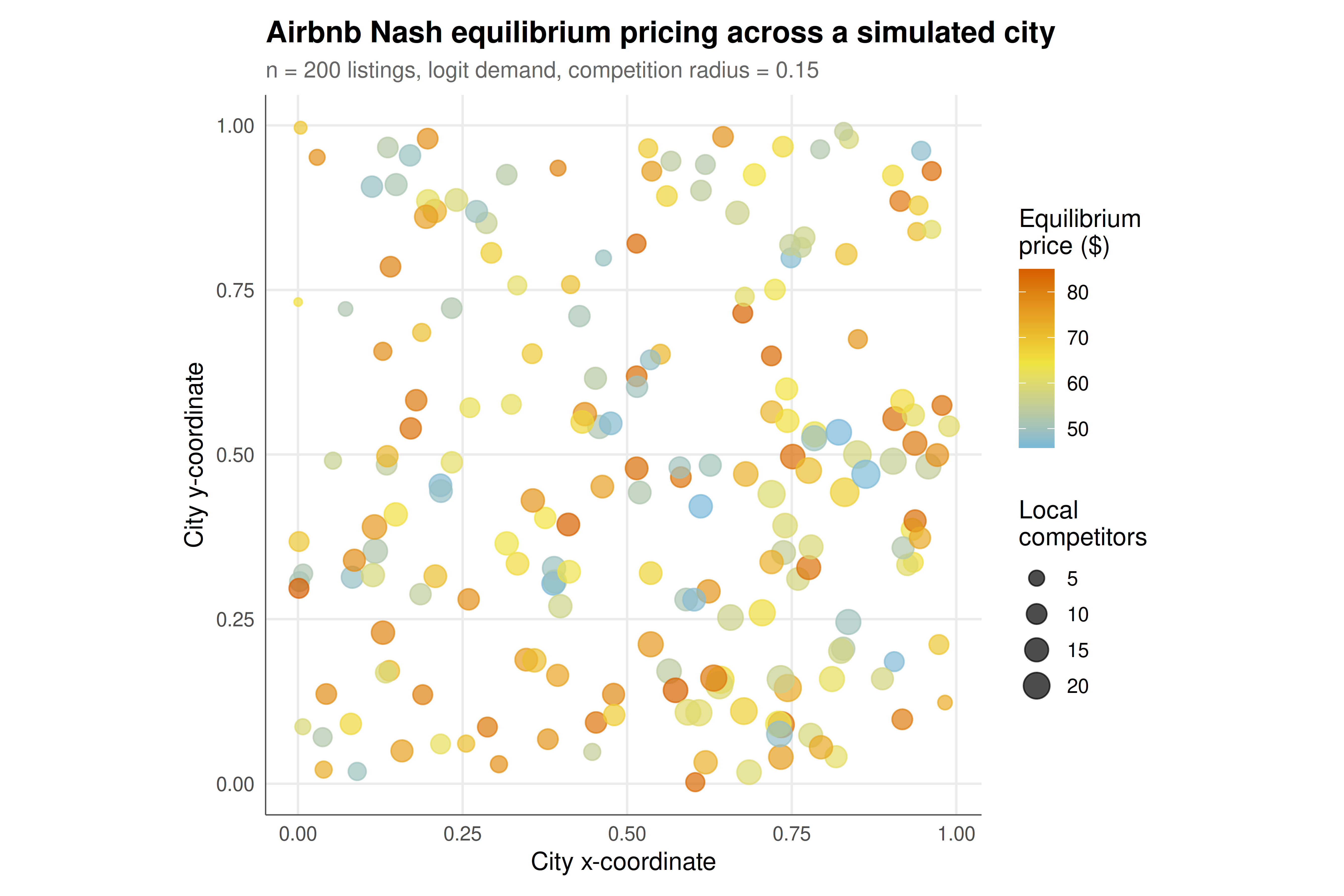
The static figure shows the spatial distribution of listings colored by equilibrium price, with point size indicating the number of local competitors.
```{r}
#| label: fig-airbnb-static
#| fig-cap: "Figure 1. Spatial distribution of 200 simulated Airbnb listings with Nash equilibrium prices computed via iterated best response in a localized logit competition model. Point color indicates the equilibrium nightly price, while point size reflects the number of competitors within the local market radius. Listings in dense areas face more competition and lower markups, while isolated premium listings command higher prices. Simulated city grid with heterogeneous listing quality. Okabe-Ito palette."
#| dev: [png, pdf]
#| fig-width: 9
#| fig-height: 6
#| dpi: 300
p_static <- ggplot(listings, aes(x = x, y = y)) +
  geom_point(aes(color = eq_price, size = n_competitors), alpha = 0.7) +
  scale_color_gradient2(
    low = okabe_ito[2], mid = okabe_ito[4], high = okabe_ito[6],
    midpoint = median(listings$eq_price),
    name = "Equilibrium\nprice ($)"
  ) +
  scale_size_continuous(range = c(1.5, 6), name = "Local\ncompetitors") +
  labs(
    title = "Airbnb Nash equilibrium pricing across a simulated city",
    subtitle = sprintf("n = %d listings, logit demand, competition radius = %.2f",
                       n_listings, radius),
    x = "City x-coordinate",
    y = "City y-coordinate"
  ) +
  theme_publication() +
  theme(legend.position = "right") +
  coord_fixed(ratio = 1)

p_static
```
## Interactive figure
The interactive version allows users to hover over individual listings to inspect their equilibrium price, quality, cost, and competitive environment.
```{r}
#| label: fig-airbnb-interactive
listings_int <- listings |>
  mutate(
    text = paste0(
      "Listing #", id,
      "\nType: ", type,
      "\nPrice: $", sprintf("%.0f", eq_price),
      "\nQuality: ", sprintf("%.1f", quality),
      "\nCost: $", sprintf("%.0f", cost),
      "\nMarkup: $", sprintf("%.0f", markup),
      "\nCompetitors: ", n_competitors,
      "\nDemand prob: ", sprintf("%.3f", demand)
    )
  )

p_int <- ggplot(listings_int, aes(x = x, y = y, color = eq_price,
                                   size = n_competitors, text = text)) +
  geom_point(alpha = 0.7) +
  scale_color_gradient2(
    low = okabe_ito[2], mid = okabe_ito[4], high = okabe_ito[6],
    midpoint = median(listings$eq_price), name = "Price ($)"
  ) +
  scale_size_continuous(range = c(1.5, 5), name = "Competitors") +
  labs(title = "Interactive Airbnb pricing map",
       x = "x", y = "y") +
  theme_publication() +
  theme(legend.position = "right") +
  coord_fixed(ratio = 1)

ggplotly(p_int, tooltip = "text") |>
  config(displaylogo = FALSE,
         modeBarButtonsToRemove = c("select2d", "lasso2d"))
```
## Interpretation
The equilibrium pricing results reveal the fundamental tension between market power and competitive pressure in localized Airbnb markets. Premium listings -- those with high quality scores reflecting superior locations, amenities, or reviews -- command significantly higher equilibrium prices than standard or budget alternatives. This premium reflects genuine differentiation: a high-quality listing attracts guests even at higher prices because the quality-adjusted utility remains competitive.
However, the spatial dimension introduces a crucial moderating factor: local density. A premium listing surrounded by many competitors within the market radius faces more competitive pressure than an equally high-quality listing in a less dense area. The equilibrium pricing formula makes this precise: the markup $p_i^* - c_i = \mu / (1 - D_i)$ is inversely related to the listing's market share $D_i$. In dense areas where many competitors split the market, each listing's share is small, pushing the markup toward $\mu$ (the minimum markup for a listing with negligible market share). In sparse areas where a listing faces few or no competitors, market share approaches its maximum, and the markup can become very large.
This density-markup relationship has practical implications for Airbnb hosts. Hosts considering entering a market should evaluate not just the average price level but the local competitive density. A neighborhood with high average prices but high density may offer lower profits than a neighborhood with moderate prices but few competitors. The game-theoretic framework quantifies this tradeoff through the equilibrium computation.
The iterated best-response algorithm we used to compute the equilibrium provides insight into the dynamic pricing process. Starting from initial prices, each host adjusts its price to maximize profit given its competitors' current prices, then the process repeats. The convergence to equilibrium in our simulation (typically within 50 to 150 iterations) corresponds to the real-world observation that Airbnb prices in active markets reach a relatively stable pattern within a few weeks of adjustment, with hosts monitoring competitors and making incremental changes.
Several model extensions would bring the analysis closer to real market conditions. First, temporal dynamics: Airbnb demand varies by season, day of week, and local events, creating time-varying games where equilibrium prices shift throughout the year. Second, capacity constraints: unlike the classical Bertrand model where a firm can serve the entire market, an Airbnb listing can host only one booking at a time, introducing capacity considerations that affect pricing strategy. Third, information asymmetry: hosts may not know competitors' costs or quality precisely, leading to games of incomplete information where Bayesian equilibrium concepts are more appropriate. Fourth, platform effects: Airbnb's search algorithm, which ranks listings based on price, quality, and responsiveness, adds a layer of platform-mediated competition that the game-theoretic framework should incorporate.
The logit demand model we employed is widely used in industrial organization because it produces well-behaved best-response functions and guarantees the existence and uniqueness of a Nash equilibrium (under mild regularity conditions). The scale parameter $\mu$ governs the intensity of competition: small $\mu$ makes consumers very price-sensitive, driving equilibrium prices toward marginal cost, while large $\mu$ gives each listing substantial market power even in competitive environments.
## Extensions & related tutorials
Airbnb pricing strategy connects to several areas of applied game theory, from spatial competition models to dynamic pricing algorithms and empirical industrial organization methods.
- [Granger causality in strategic interactions](../../time-series-econometrics/granger-causality-strategic/)
- [Bootstrap methods for game-theoretic inference](../../statistical-foundations/bootstrap-methods-game-theory/)
- [Agent-based modeling for game theory in R](../../simulations/agent-based-modeling-netlogo-style/)
- [Interactive dashboards for game theory with flexdashboard](../../visualization-and-communication/dashboard-flexdashboard-games/)
- [Docker containers for reproducible game theory analysis](../../reproducibility-open-science/docker-reproducible-game-analysis/)
## References
::: {#refs}
:::