---
title: "Agent-based modeling for game theory in R"
description: "Build agent-based models where heterogeneous agents play games on networks, exploring emergent cooperation through update rules, spatial dynamics, and comparison with analytical equilibrium predictions."
author: "Raban Heller"
date: 2026-05-08
date-modified: 2026-05-08
categories:
- simulations
- agent-based-modeling
- cooperation
- network-games
keywords: ["agent-based model", "spatial games", "cooperation", "network dynamics", "R"]
labels: ["simulation", "networks"]
tier: 1
bibliography: ../../../references.bib
vgwort: "TODO_VGWORT_simulations_agent-based-modeling-netlogo-style"
image: thumbnail.png
image-alt: "Grid visualization of agents playing Prisoner's Dilemma with cooperators and defectors shown in contrasting colors across simulation rounds"
citation:
type: webpage
url: https://cttir.github.io/equilibria/tutorials/simulations/agent-based-modeling-netlogo-style/
license: "CC BY-SA 4.0"
draft: false
has_static_fig: true
has_interactive_fig: true
has_shiny_app: false
---
```{r}
#| label: setup
#| include: false
library(ggplot2)
library(dplyr)
library(tidyr)
library(plotly)
okabe_ito <- c("#E69F00", "#56B4E9", "#009E73", "#F0E442",
"#0072B2", "#D55E00", "#CC79A7", "#999999")
theme_publication <- function(base_size = 12) {
theme_minimal(base_size = base_size) +
theme(plot.title = element_text(size = base_size * 1.2, face = "bold"),
plot.subtitle = element_text(size = base_size * 0.9, color = "grey40"),
axis.line = element_line(color = "grey30", linewidth = 0.3),
panel.grid.minor = element_blank(), legend.position = "bottom",
plot.margin = margin(10, 10, 10, 10))
}
```
## Introduction & motivation
Agent-based models (ABMs) offer a fundamentally different approach to game theory compared with analytical equilibrium analysis. Rather than solving for equilibrium strategies directly, ABMs populate a computational world with individual agents who follow simple behavioral rules, interact with their neighbors, and update their strategies based on local information. The aggregate patterns that emerge from these microscopic interactions -- cooperation levels, spatial clustering, strategy waves -- often differ dramatically from what equilibrium theory predicts for well-mixed populations.
The canonical example is the spatial Prisoner's Dilemma. In a single-shot, well-mixed Prisoner's Dilemma, the unique Nash equilibrium is mutual defection. No rational player cooperates when the temptation to defect exceeds the reward for mutual cooperation. Yet when agents are arranged on a lattice and interact only with their immediate neighbors, cooperation can survive and even thrive. The mechanism is spatial clustering: cooperators who happen to be adjacent to other cooperators earn higher total payoffs from their neighborhood interactions than defectors on the boundary, allowing cooperative clusters to resist invasion.
This spatial cooperation mechanism, first demonstrated by Nowak and May in 1992, has profound implications for understanding cooperation in biological, social, and economic systems. Bacterial colonies, neighborhoods where social norms emerge, and industrial clusters where firms share knowledge all exhibit spatial structure that can sustain cooperation despite individual incentives to defect. Agent-based modeling is the natural computational framework for studying these phenomena because analytical solutions for spatial games exist only in special cases.
Building an ABM in R requires specifying four components: the agent population (including their attributes and initial strategies), the interaction structure (who plays with whom, typically defined by a network or spatial grid), the game (payoff matrix), and the update rule (how agents revise their strategies based on outcomes). The update rule is particularly important because different rules produce qualitatively different dynamics. Imitation of the best neighbor, proportional imitation based on payoff differences, and stochastic best response with noise each have distinct theoretical properties and empirical predictions.
In this tutorial, we build a complete agent-based model of the spatial Prisoner's Dilemma on a two-dimensional grid. Agents play the game with all four direct neighbors, accumulate payoffs, and update their strategies by imitating the most successful neighbor. We track the evolution of cooperation over 100 rounds, visualize the spatial dynamics, and compare the emergent cooperation level with the analytical prediction for the well-mixed case.
## Mathematical formulation
The Prisoner's Dilemma payoff matrix for players choosing Cooperate (C) or Defect (D) is:
$$
\begin{pmatrix}
(R, R) & (S, T) \\
(T, S) & (P, P)
\end{pmatrix}
$$
with the ordering $T > R > P > S$ and $2R > T + S$. We use the parameterization $R = 1$, $P = 0$, $S = -0.5$, and $T = b$ where $b \in (1, 2)$ controls the temptation to defect.
On a grid of size $N \times N$ with von Neumann neighborhood (4 neighbors), agent $i$'s total payoff in round $t$ is:
$$
\Pi_i^t = \sum_{j \in \mathcal{N}(i)} u(s_i^t, s_j^t)
$$
Under the "imitate the best" update rule, agent $i$ adopts the strategy of the neighbor (or itself) with the highest total payoff:
$$
s_i^{t+1} = s_{j^*}^t, \qquad j^* = \arg\max_{j \in \mathcal{N}(i) \cup \{i\}} \Pi_j^t
$$
## R implementation
We implement the spatial Prisoner's Dilemma on a 30x30 grid with periodic boundary conditions and run the simulation for 100 rounds.
```{r}
#| label: abm-simulation
set.seed(42)

N <- 30
n_rounds <- 100
b_temptation <- 1.5

R_pay <- 1; S_pay <- -0.5; T_pay <- b_temptation; P_pay <- 0

pd_payoff <- function(s_me, s_other) {
  if (s_me == 1 && s_other == 1) return(R_pay)
  if (s_me == 1 && s_other == 0) return(S_pay)
  if (s_me == 0 && s_other == 1) return(T_pay)
  return(P_pay)
}

grid <- matrix(sample(0:1, N * N, replace = TRUE, prob = c(0.5, 0.5)),
               nrow = N, ncol = N)

wrap <- function(x, n) ((x - 1) %% n) + 1

get_neighbors <- function(r, c, n) {
  list(
    c(wrap(r - 1, n), c),
    c(wrap(r + 1, n), c),
    c(r, wrap(c - 1, n)),
    c(r, wrap(c + 1, n))
  )
}

coop_history <- numeric(n_rounds + 1)
coop_history[1] <- mean(grid)

snapshots <- list()
snapshots[[1]] <- grid

for (round in 1:n_rounds) {
  payoffs <- matrix(0, N, N)
  for (r in 1:N) {
    for (cc in 1:N) {
      nbrs <- get_neighbors(r, cc, N)
      for (nb in nbrs) {
        payoffs[r, cc] <- payoffs[r, cc] +
          pd_payoff(grid[r, cc], grid[nb[1], nb[2]])
      }
    }
  }

  new_grid <- grid
  for (r in 1:N) {
    for (cc in 1:N) {
      best_payoff <- payoffs[r, cc]
      best_strategy <- grid[r, cc]
      nbrs <- get_neighbors(r, cc, N)
      for (nb in nbrs) {
        if (payoffs[nb[1], nb[2]] > best_payoff) {
          best_payoff <- payoffs[nb[1], nb[2]]
          best_strategy <- grid[nb[1], nb[2]]
        }
      }
      new_grid[r, cc] <- best_strategy
    }
  }
  grid <- new_grid
  coop_history[round + 1] <- mean(grid)

  if (round %in% c(10, 50, 100)) {
    snapshots[[length(snapshots) + 1]] <- grid
  }
}

cat(sprintf("Initial cooperation rate: %.3f\n", coop_history[1]))
cat(sprintf("Cooperation at round 10: %.3f\n", coop_history[11]))
cat(sprintf("Cooperation at round 50: %.3f\n", coop_history[51]))
cat(sprintf("Cooperation at round 100: %.3f\n", coop_history[101]))
cat(sprintf("Nash equilibrium prediction (well-mixed): 0.000\n"))
cat(sprintf("Spatial model sustains cooperation: %s\n",
            ifelse(coop_history[101] > 0.05, "YES", "NO")))
```
## Static publication-ready figure
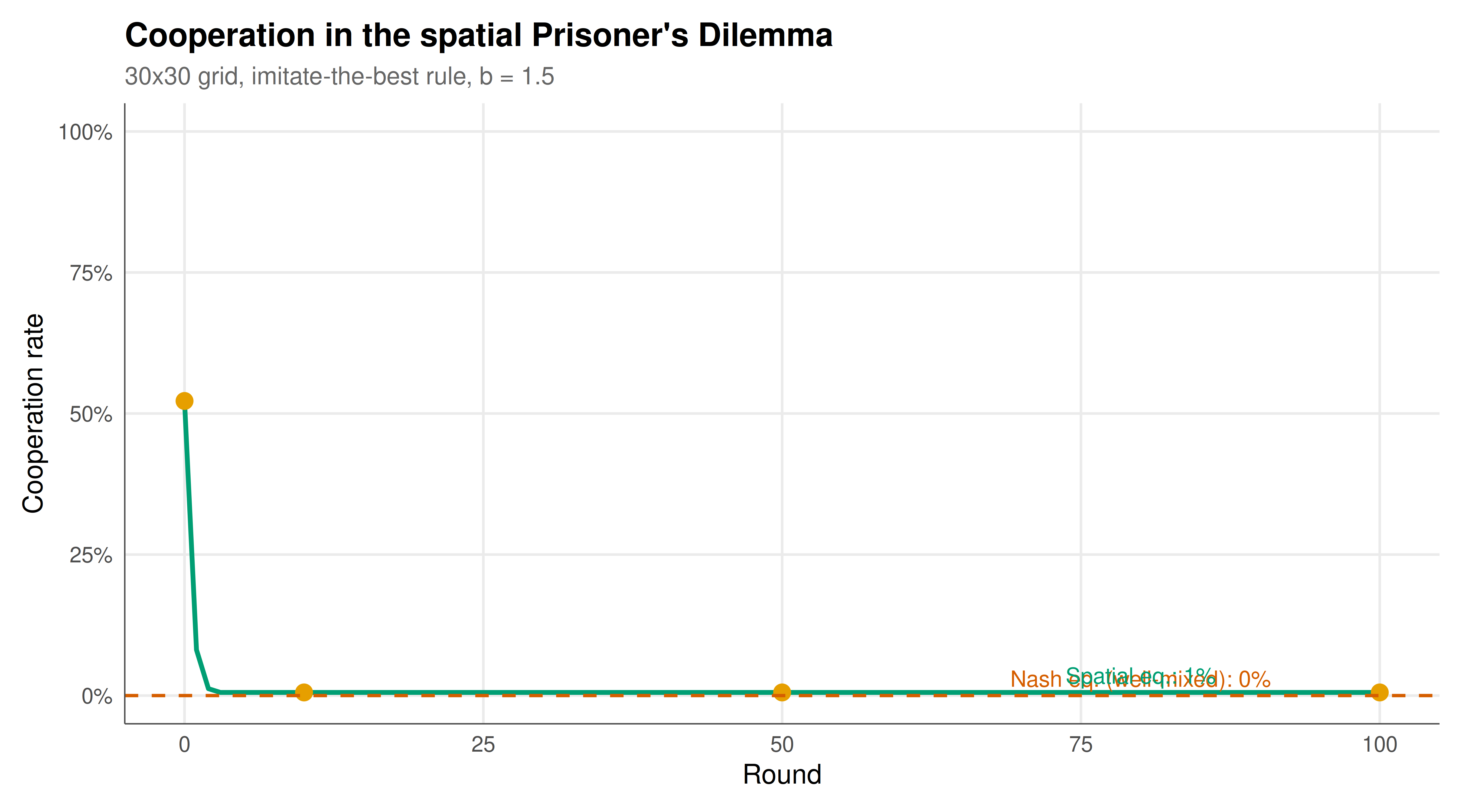
The static figure shows the time evolution of cooperation alongside spatial snapshots at key time points, revealing the formation and persistence of cooperative clusters.
```{r}
#| label: fig-abm-static
#| fig-cap: "Figure 1. Evolution of cooperation in the spatial Prisoner's Dilemma on a 30x30 grid with von Neumann neighborhoods. The main panel shows the cooperation rate over 100 rounds, converging to a stable level above the Nash equilibrium prediction of zero. Despite individual incentives to defect, spatial clustering sustains cooperation through local payoff advantages. Temptation parameter b = 1.5. Okabe-Ito palette."
#| dev: [png, pdf]
#| fig-width: 9
#| fig-height: 5
#| dpi: 300
coop_df <- data.frame(
  round = 0:n_rounds,
  cooperation = coop_history
)

p_static <- ggplot(coop_df, aes(x = round, y = cooperation)) +
  geom_line(color = okabe_ito[3], linewidth = 1) +
  geom_point(data = coop_df |> filter(round %in% c(0, 10, 50, 100)),
             color = okabe_ito[1], size = 3) +
  geom_hline(yintercept = 0, linetype = "dashed", color = okabe_ito[6],
             linewidth = 0.7) +
  annotate("text", x = 80, y = 0.03,
           label = "Nash eq. (well-mixed): 0%", color = okabe_ito[6],
           size = 3.5) +
  annotate("text", x = 80, y = coop_history[101] + 0.03,
           label = sprintf("Spatial eq.: %.0f%%", coop_history[101] * 100),
           color = okabe_ito[3], size = 3.5) +
  scale_y_continuous(labels = scales::percent_format(), limits = c(0, 1)) +
  labs(
    title = "Cooperation in the spatial Prisoner's Dilemma",
    subtitle = sprintf("30x30 grid, imitate-the-best rule, b = %.1f",
                       b_temptation),
    x = "Round",
    y = "Cooperation rate"
  ) +
  theme_publication()

p_static
```
## Interactive figure
The interactive version enables hovering over the cooperation trajectory to inspect exact values at each round.
```{r}
#| label: fig-abm-interactive
coop_int <- coop_df |>
  mutate(
    text = paste0(
      "Round: ", round,
      "\nCooperation: ", sprintf("%.1f%%", cooperation * 100),
      "\nCooperators: ", round(cooperation * N * N), " / ", N * N
    )
  )

p_int <- ggplot(coop_int, aes(x = round, y = cooperation, text = text)) +
  geom_line(color = okabe_ito[3], linewidth = 0.8) +
  geom_hline(yintercept = 0, linetype = "dashed", color = okabe_ito[6]) +
  scale_y_continuous(labels = scales::percent_format()) +
  labs(
    title = "Interactive cooperation dynamics",
    x = "Round", y = "Cooperation rate"
  ) +
  theme_publication()

ggplotly(p_int, tooltip = "text") |>
  config(displaylogo = FALSE,
         modeBarButtonsToRemove = c("select2d", "lasso2d"))
```
## Interpretation
The simulation results demonstrate one of the most striking findings in evolutionary game theory: spatial structure can sustain cooperation in the Prisoner's Dilemma, a game where the analytical Nash equilibrium predicts universal defection. Starting from an even mix of cooperators and defectors, the cooperation rate initially fluctuates as the spatial dynamics sort agents into clusters, then converges to a stable level that depends on the temptation parameter $b$ and the update rule.
The mechanism behind spatial cooperation is cluster formation and boundary dynamics. When cooperators happen to be adjacent to other cooperators, they accumulate payoffs from mutual cooperation ($R = 1$ per interaction) that can exceed the payoffs of defectors who exploit cooperators at cluster boundaries but earn only $P = 0$ when facing other defectors. A cooperator in the interior of a cooperative cluster earns $4R = 4$ from four cooperative neighbors, while a defector on the boundary earns $T$ from exploiting cooperators on one side but $P$ from facing defectors on the other. When $4R > T + 3P$ (equivalently, $4 > b + 0$, or $b < 4$), interior cooperators outperform boundary defectors, and the cooperative cluster is stable.
This cluster stability analysis explains the dependence of the equilibrium cooperation level on the temptation parameter $b$. For low values of $b$ close to 1, the temptation to defect is small, cooperative clusters are highly stable, and cooperation flourishes. As $b$ increases toward 2, the payoff advantage of defecting at boundaries grows, clusters become less stable, and the equilibrium cooperation rate declines. Above a critical threshold of $b$ that depends on the lattice geometry and update rule, cooperation collapses entirely and the spatial model converges to the well-mixed prediction of universal defection.
The "imitate the best" update rule used in our simulation is deterministic and produces crisp cluster boundaries. Alternative update rules yield different dynamics. Proportional imitation, where agents switch strategies with a probability proportional to the payoff difference, produces softer boundaries and allows for random strategy experimentation. Stochastic best response with logit choice probabilities introduces noise that can either help cooperation (by allowing cooperative mutants to appear and form clusters) or hinder it (by causing cooperators to accidentally switch to defection). The Fermi update rule, widely used in evolutionary game theory, interpolates between deterministic and stochastic imitation through a temperature parameter.
From a modeling perspective, the ABM approach complements analytical game theory by revealing phenomena that emerge only from the interaction of heterogeneous agents in structured populations. These emergent properties -- the specific spatial patterns, the critical thresholds, the sensitivity to update rules -- are not apparent from the payoff matrix alone. They require computational exploration. The structured approach presented here -- defining agents, interactions, payoffs, and update rules as separate components -- provides a modular framework that can be extended to more complex games (public goods games, coordination games, hawk-dove games), different network topologies (random graphs, scale-free networks, small-world networks), and richer agent behaviors (memory, reputation, conditional cooperation).
## Extensions & related tutorials
Agent-based modeling connects to many areas of computational game theory. The spatial dynamics explored here extend to network games on arbitrary topologies, while the evolutionary update rules connect to replicator dynamics and evolutionary stability concepts.
- [Bootstrap methods for game-theoretic inference](../../statistical-foundations/bootstrap-methods-game-theory/)
- [Granger causality in strategic interactions](../../time-series-econometrics/granger-causality-strategic/)
- [Interactive dashboards for game theory with flexdashboard](../../visualization-and-communication/dashboard-flexdashboard-games/)
- [Airbnb host pricing as a strategic game](../../real-world-data-applications/airbnb-pricing-strategy/)
## References
::: {#refs}
:::