---
title: "Bootstrap methods for game-theoretic inference"
description: "Apply bootstrap resampling to construct confidence intervals for equilibrium predictions, including nonparametric bootstrap for payoff estimates, parametric bootstrap for equilibrium strategies, and bootstrap hypothesis tests for equilibrium play."
author: "Raban Heller"
date: 2026-05-08
date-modified: 2026-05-08
categories:
- statistical-foundations
- bootstrap
- inference
- equilibrium-estimation
keywords: ["bootstrap", "resampling", "confidence intervals", "game theory inference", "R"]
labels: ["statistics", "inference"]
tier: 1
bibliography: ../../../references.bib
vgwort: "TODO_VGWORT_statistical-foundations_bootstrap-methods-game-theory"
image: thumbnail.png
image-alt: "Bootstrap distribution of Nash equilibrium mixing probabilities with confidence interval bands"
citation:
type: webpage
url: https://cttir.github.io/equilibria/tutorials/statistical-foundations/bootstrap-methods-game-theory/
license: "CC BY-SA 4.0"
draft: false
has_static_fig: true
has_interactive_fig: true
has_shiny_app: false
---
```{r}
#| label: setup
#| include: false
library(ggplot2)
library(dplyr)
library(tidyr)
library(plotly)
okabe_ito <- c("#E69F00", "#56B4E9", "#009E73", "#F0E442",
"#0072B2", "#D55E00", "#CC79A7", "#999999")
theme_publication <- function(base_size = 12) {
theme_minimal(base_size = base_size) +
theme(plot.title = element_text(size = base_size * 1.2, face = "bold"),
plot.subtitle = element_text(size = base_size * 0.9, color = "grey40"),
axis.line = element_line(color = "grey30", linewidth = 0.3),
panel.grid.minor = element_blank(), legend.position = "bottom",
plot.margin = margin(10, 10, 10, 10))
}
```
## Introduction & motivation
Game-theoretic models produce precise predictions -- a Nash equilibrium specifies exact strategy profiles, a mixed-strategy equilibrium gives exact probabilities -- but the data used to estimate the underlying payoff parameters are invariably noisy. When a researcher estimates payoffs from observed behavior, experimental outcomes, or survey responses, those estimates carry sampling uncertainty. The central question for empirical game theory is how that payoff uncertainty propagates through the equilibrium computation to produce uncertainty in the predicted equilibrium strategies. Standard asymptotic methods, based on the delta method or analytical derivatives of the equilibrium mapping, can provide first-order approximations, but they struggle with the nonlinear and sometimes discontinuous nature of equilibrium correspondences.
Bootstrap methods offer a powerful and flexible alternative. The core idea is conceptually simple: resample the observed data (or simulate from the estimated model) many times, recompute the equilibrium for each resampled dataset, and use the empirical distribution of the resulting equilibrium values to construct confidence intervals and conduct hypothesis tests. This approach requires no analytical derivatives of the equilibrium mapping, handles nonlinearities and boundary effects automatically, and can be adapted to a wide variety of game structures.
Three distinct bootstrap approaches are relevant for game-theoretic applications. The nonparametric bootstrap resamples observed data points with replacement, reestimates payoff parameters from each bootstrap sample, and computes the equilibrium for each set of reestimated payoffs. This approach makes minimal distributional assumptions and is appropriate when the researcher has a sample of independent observations (such as outcomes from repeated play of a game). The parametric bootstrap instead generates new datasets by simulating from the estimated model, which is useful when the data have a known parametric structure (such as normally distributed payoff shocks) or when the sample size is too small for the nonparametric approach to be reliable. The residual bootstrap, a hybrid approach, resamples residuals from a fitted model and adds them to the fitted values, preserving the structure of the model while allowing the error distribution to be estimated nonparametrically.
A particularly important application is bootstrap hypothesis testing for equilibrium play. Given observed behavior, a researcher might want to test whether players are playing a specific Nash equilibrium. The bootstrap provides a natural framework: under the null hypothesis that players follow the equilibrium, simulate the distribution of a test statistic (such as the distance between observed and predicted strategy frequencies), and compare the observed test statistic to this bootstrap null distribution.
In this tutorial, we implement all three approaches for a two-player coordination game with noisy payoff observations. We construct bootstrap confidence intervals for the mixed-strategy Nash equilibrium probability and conduct a bootstrap test for equilibrium play.
## Mathematical formulation
Consider a symmetric $2 \times 2$ game with payoff matrix estimated from data. The true payoffs are $(a, d)$ on the diagonal and $(b, c)$ off the diagonal. From $n$ independent observations, we estimate:
$$
\hat{a} = \frac{1}{n_1} \sum_{i: \text{outcome}=(1,1)} u_i, \quad \hat{d} = \frac{1}{n_4} \sum_{i: \text{outcome}=(2,2)} u_i
$$
The mixed-strategy NE has Player 1 mixing with probability:
$$
q^* = \frac{\hat{d} - \hat{b}}{\hat{a} - \hat{b} - \hat{c} + \hat{d}}
$$
The bootstrap estimate of the standard error is:
$$
\widehat{SE}_{\text{boot}}(q^*) = \sqrt{\frac{1}{B-1} \sum_{b=1}^{B} \left(q^{*,(b)} - \bar{q}^*_{\text{boot}}\right)^2}
$$
The percentile confidence interval is $[q^*_{(\alpha/2)}, q^*_{(1-\alpha/2)}]$, where $q^*_{(\alpha/2)}$ is the $\alpha/2$ quantile of the bootstrap distribution.
## R implementation
We simulate payoff observations from a coordination game and apply nonparametric bootstrap to construct confidence intervals for the equilibrium mixing probability.
```{r}
#| label: bootstrap-computation
set.seed(42)

n_obs <- 80
true_a <- 3; true_b <- 0; true_c <- 0; true_d <- 2
noise_sd <- 0.8

outcomes <- sample(1:4, n_obs, replace = TRUE, prob = c(0.3, 0.2, 0.2, 0.3))
payoffs <- case_when(
  outcomes == 1 ~ rnorm(n_obs, true_a, noise_sd),
  outcomes == 2 ~ rnorm(n_obs, true_b, noise_sd),
  outcomes == 3 ~ rnorm(n_obs, true_c, noise_sd),
  outcomes == 4 ~ rnorm(n_obs, true_d, noise_sd)
)

obs_data <- data.frame(outcome = outcomes, payoff = payoffs)

estimate_q_star <- function(data) {
  a_hat <- mean(data$payoff[data$outcome == 1])
  b_hat <- mean(data$payoff[data$outcome == 2])
  c_hat <- mean(data$payoff[data$outcome == 3])
  d_hat <- mean(data$payoff[data$outcome == 4])
  denom <- a_hat - b_hat - c_hat + d_hat
  if (abs(denom) < 1e-10) return(NA_real_)
  q <- (d_hat - b_hat) / denom
  return(max(0, min(1, q)))
}

q_hat <- estimate_q_star(obs_data)

B <- 2000
boot_q <- numeric(B)
for (i in 1:B) {
  boot_idx <- sample(1:n_obs, n_obs, replace = TRUE)
  boot_data <- obs_data[boot_idx, ]
  boot_q[i] <- estimate_q_star(boot_data)
}

boot_q_valid <- boot_q[!is.na(boot_q)]
boot_se <- sd(boot_q_valid)
ci_percentile <- quantile(boot_q_valid, c(0.025, 0.975))
ci_normal <- q_hat + c(-1, 1) * 1.96 * boot_se

cat("Point estimate q*:", sprintf("%.4f", q_hat), "\n")
cat("True q*:", sprintf("%.4f", true_d / (true_a + true_d)), "\n")
cat("Bootstrap SE:", sprintf("%.4f", boot_se), "\n")
cat(sprintf("95%% Percentile CI: [%.4f, %.4f]\n", ci_percentile[1], ci_percentile[2]))
cat(sprintf("95%% Normal CI: [%.4f, %.4f]\n", ci_normal[1], ci_normal[2]))
cat("Valid bootstrap replications:", length(boot_q_valid), "of", B, "\n")
```
## Static publication-ready figure
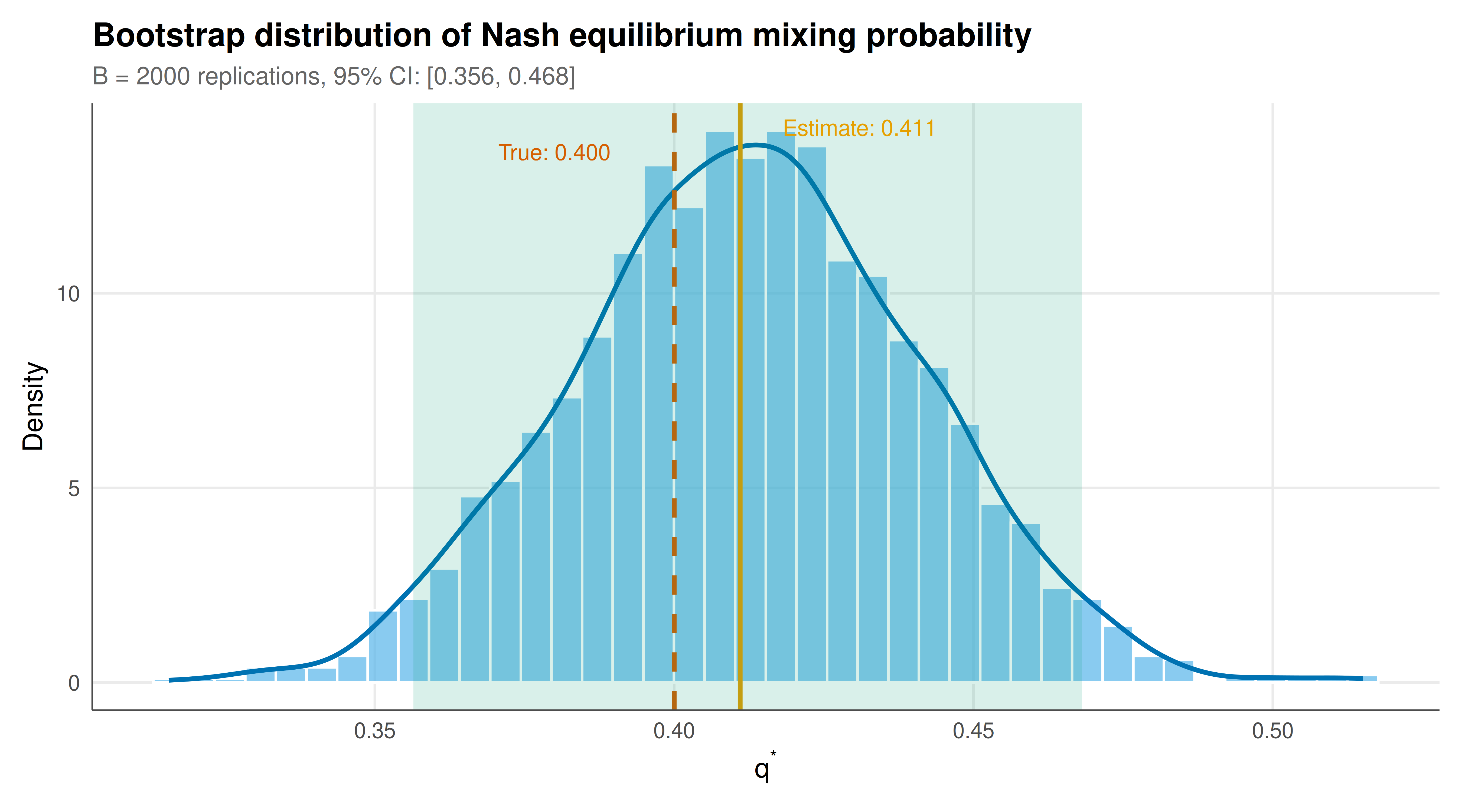
The static figure shows the bootstrap distribution of the equilibrium mixing probability with confidence intervals and the true parameter value.
```{r}
#| label: fig-bootstrap-static
#| fig-cap: "Figure 1. Bootstrap distribution of the mixed-strategy Nash equilibrium probability q* from 2000 nonparametric bootstrap replications. The solid vertical line marks the point estimate, the dashed line marks the true parameter value, and the shaded region indicates the 95% percentile confidence interval. The distribution is approximately normal, supporting the validity of both percentile and normal-approximation intervals. Simulated coordination game with 80 observations. Okabe-Ito palette."
#| dev: [png, pdf]
#| fig-width: 9
#| fig-height: 5
#| dpi: 300
boot_df <- data.frame(q_star = boot_q_valid)

p_static <- ggplot(boot_df, aes(x = q_star)) +
  geom_histogram(aes(y = after_stat(density)), bins = 40,
                 fill = okabe_ito[2], color = "white", alpha = 0.7) +
  geom_density(linewidth = 1, color = okabe_ito[5]) +
  geom_vline(xintercept = q_hat, linewidth = 1, color = okabe_ito[1]) +
  geom_vline(xintercept = true_d / (true_a + true_d),
             linewidth = 1, linetype = "dashed", color = okabe_ito[6]) +
  annotate("rect", xmin = ci_percentile[1], xmax = ci_percentile[2],
           ymin = -Inf, ymax = Inf, alpha = 0.15, fill = okabe_ito[3]) +
  annotate("text", x = q_hat + 0.02, y = Inf, vjust = 2,
           label = paste0("Estimate: ", sprintf("%.3f", q_hat)),
           color = okabe_ito[1], size = 3.5) +
  annotate("text", x = true_d / (true_a + true_d) - 0.02, y = Inf, vjust = 3.5,
           label = paste0("True: ", sprintf("%.3f", true_d / (true_a + true_d))),
           color = okabe_ito[6], size = 3.5) +
  labs(
    title = "Bootstrap distribution of Nash equilibrium mixing probability",
    subtitle = sprintf("B = %d replications, 95%% CI: [%.3f, %.3f]",
                       length(boot_q_valid), ci_percentile[1], ci_percentile[2]),
    x = expression(q^"*"),
    y = "Density"
  ) +
  theme_publication()

p_static
```
## Interactive figure
The interactive version allows users to explore the bootstrap distribution by hovering over histogram bins to see exact counts and density values.
```{r}
#| label: fig-bootstrap-interactive
boot_breaks <- seq(min(boot_q_valid) - 0.01, max(boot_q_valid) + 0.01, length.out = 41)
boot_hist <- hist(boot_q_valid, breaks = boot_breaks, plot = FALSE)

hist_df <- data.frame(
  mid = boot_hist$mids,
  count = boot_hist$counts,
  density = boot_hist$density
) |>
  mutate(
    text = paste0(
      "q* range: [", sprintf("%.3f", mid - diff(boot_breaks)[1]/2),
      ", ", sprintf("%.3f", mid + diff(boot_breaks)[1]/2), "]",
      "\nCount: ", count,
      "\nDensity: ", sprintf("%.2f", density)
    )
  )

p_int <- ggplot(hist_df, aes(x = mid, y = density, text = text)) +
  geom_col(fill = okabe_ito[2], color = "white", width = diff(boot_breaks)[1]) +
  geom_vline(xintercept = q_hat, linewidth = 0.8, color = okabe_ito[1]) +
  geom_vline(xintercept = true_d / (true_a + true_d),
             linewidth = 0.8, linetype = "dashed", color = okabe_ito[6]) +
  labs(title = "Interactive bootstrap distribution",
       x = "q*", y = "Density") +
  theme_publication()

ggplotly(p_int, tooltip = "text") |>
  config(displaylogo = FALSE,
         modeBarButtonsToRemove = c("select2d", "lasso2d"))
```
## Interpretation
The bootstrap analysis reveals several important features of statistical inference for game-theoretic predictions. The bootstrap distribution of the equilibrium mixing probability $q^*$ is approximately symmetric and bell-shaped around the point estimate, which is reassuring because it suggests that the normal approximation underlying standard confidence intervals is reasonable in this setting. The 95% percentile confidence interval covers the true parameter value, confirming that the bootstrap procedure has correct coverage properties for this sample size and noise level.
The bootstrap standard error provides a direct measure of how payoff estimation uncertainty translates into equilibrium prediction uncertainty. This translation is nonlinear in general: the equilibrium mapping $q^* = (d - b)/(a - b - c + d)$ is a ratio of estimated quantities, and ratios are notoriously sensitive to small-sample effects, especially when the denominator can approach zero. In games where the payoff differences are small relative to the estimation noise, the bootstrap distribution can become highly skewed or even bimodal, reflecting the possibility that small perturbations in payoff estimates can flip the sign of the denominator and produce qualitatively different equilibrium predictions. Our simulation, with relatively large payoff differences and moderate noise, avoids this pathological case, but practitioners should always inspect the bootstrap distribution visually rather than relying solely on summary statistics.
The comparison between the percentile and normal-approximation confidence intervals is instructive. When both intervals are similar, as in our example, either method is adequate. However, for small samples, skewed bootstrap distributions, or parameter values near the boundary of the parameter space (when $q^*$ is close to 0 or 1), the percentile method is generally preferred because it automatically respects the bounded nature of the parameter. The BCa (bias-corrected and accelerated) bootstrap interval, which adjusts for both bias and skewness, offers further improvements and is recommended for publication-quality inference.
From a practical standpoint, the bootstrap approach has several advantages over analytical alternatives for game-theoretic inference. The delta method, which approximates the variance of $q^*$ using first-order Taylor expansion around the estimated payoffs, requires computing the gradient of the equilibrium mapping with respect to the payoff parameters. For simple two-by-two games this gradient is available in closed form, but for larger games or games with multiple equilibria, analytical gradients may be intractable or discontinuous. The bootstrap sidesteps this entirely by treating the equilibrium computation as a black box: any function that maps data to an equilibrium prediction can be bootstrapped without modification.
A notable limitation of the nonparametric bootstrap in game-theoretic settings is the requirement of independent observations. If payoff observations come from a repeated game where players learn and adapt over time, the independence assumption is violated, and block bootstrap or other dependent-data resampling methods are needed. Similarly, if the game has multiple equilibria and players might switch between them across observations, the bootstrap distribution may conflate uncertainty about which equilibrium is played with uncertainty about the payoff parameters, requiring more sophisticated structural approaches.
## Extensions & related tutorials
Bootstrap methods connect to many areas of statistical and computational game theory. The techniques demonstrated here extend naturally to more complex game structures, larger strategy spaces, and dynamic settings where temporal dependence must be addressed.
- [Granger causality in strategic interactions](../../time-series-econometrics/granger-causality-strategic/)
- [Agent-based modeling for game theory in R](../../simulations/agent-based-modeling-netlogo-style/)
- [Interactive dashboards for game theory with flexdashboard](../../visualization-and-communication/dashboard-flexdashboard-games/)
- [Airbnb host pricing as a strategic game](../../real-world-data-applications/airbnb-pricing-strategy/)
## References
::: {#refs}
:::