---
title: "Interactive dashboards for game theory with flexdashboard"
description: "Build interactive dashboards to explore game-theoretic models using flexdashboard, combining reactive inputs for payoff parameters with real-time equilibrium computation and multiple coordinated visualizations."
author: "Raban Heller"
date: 2026-05-08
date-modified: 2026-05-08
categories:
- visualization-and-communication
- dashboards
- flexdashboard
- interactive-visualization
keywords: ["flexdashboard", "interactive dashboard", "game theory visualization", "R", "Shiny"]
labels: ["visualization", "interactive"]
tier: 1
bibliography: ../../../references.bib
vgwort: "TODO_VGWORT_visualization-and-communication_dashboard-flexdashboard-games"
image: thumbnail.png
image-alt: "Dashboard layout showing game theory payoff matrices and equilibrium regions with interactive controls"
citation:
type: webpage
url: https://cttir.github.io/equilibria/tutorials/visualization-and-communication/dashboard-flexdashboard-games/
license: "CC BY-SA 4.0"
draft: false
has_static_fig: true
has_interactive_fig: true
has_shiny_app: false
---
```{r}
#| label: setup
#| include: false
library(ggplot2)
library(dplyr)
library(tidyr)
library(plotly)
okabe_ito <- c("#E69F00", "#56B4E9", "#009E73", "#F0E442",
"#0072B2", "#D55E00", "#CC79A7", "#999999")
theme_publication <- function(base_size = 12) {
theme_minimal(base_size = base_size) +
theme(plot.title = element_text(size = base_size * 1.2, face = "bold"),
plot.subtitle = element_text(size = base_size * 0.9, color = "grey40"),
axis.line = element_line(color = "grey30", linewidth = 0.3),
panel.grid.minor = element_blank(), legend.position = "bottom",
plot.margin = margin(10, 10, 10, 10))
}
```
## Introduction & motivation
Game theory produces rich analytical results, but communicating those results to diverse audiences -- students, policymakers, business strategists -- remains a persistent challenge. A static payoff matrix or a single equilibrium diagram captures one configuration of a game, yet the real insight often lies in understanding how equilibria shift as parameters change. When a student adjusts a discount factor and watches a cooperation region expand in real time, the intuition behind the folk theorem becomes visceral rather than abstract. When a consultant lets a client drag a slider for market entry cost and sees the Nash equilibrium price jump discontinuously, the strategic implications of sunk costs are immediately apparent.
Interactive dashboards address this communication gap by turning analytical models into explorable interfaces. The R ecosystem offers several frameworks for building such dashboards, and flexdashboard stands out for game-theoretic applications because of its simplicity of layout specification, native integration with R Markdown, and the ability to add Shiny reactivity without requiring a standalone server application. A flexdashboard document is essentially an R Markdown file with a special output format that arranges content into rows and columns, value boxes, and tabbed panels. When combined with Shiny runtime, inputs such as sliders, dropdowns, and numeric fields can drive reactive computations that update plots and tables whenever the user changes a parameter.
In this tutorial, we focus on the design principles and computational patterns that make game-theoretic dashboards effective, rather than deploying a live flexdashboard (which requires a Shiny server). We will build the core components -- payoff parameter grids, equilibrium computation functions, and coordinated multi-panel visualizations -- that form the backbone of any such dashboard. The approach generalizes: whether you are visualizing a simple two-by-two game, a Cournot oligopoly with variable numbers of firms, or a repeated game with discounting, the pattern of parameter input, equilibrium computation, and result display remains the same.
The design philosophy we adopt here follows established principles from information visualization research. We use small multiples to compare equilibrium regions across parameter ranges, coordinated views so that highlighting one region in payoff space simultaneously highlights the corresponding strategy profile, and progressive disclosure so that a summary view is available at a glance while detailed breakdowns are accessible on demand. These principles ensure that the dashboard is not merely a collection of widgets but a coherent analytical tool.
Throughout this article, we simulate the dashboard components as static and interactive R outputs. The code is structured so that wrapping these components in a flexdashboard layout with Shiny reactivity requires only minor modifications -- replacing fixed parameter values with input widget references and wrapping plot code in render functions.
## Mathematical formulation
We consider a general two-player normal-form game with parameterized payoffs. Player 1 chooses from strategies $\{s_1^1, s_1^2\}$ and Player 2 from $\{s_2^1, s_2^2\}$. The payoff matrix is:
$$
\begin{pmatrix}
(a, e) & (b, f) \\
(c, g) & (d, h)
\end{pmatrix}
$$
where $a, b, c, d$ are Player 1's payoffs and $e, f, g, h$ are Player 2's payoffs. A pure-strategy Nash equilibrium $(s_1^i, s_2^j)$ satisfies:
$$
u_1(s_1^i, s_2^j) \geq u_1(s_1^k, s_2^j) \quad \forall k, \qquad u_2(s_1^i, s_2^j) \geq u_2(s_1^i, s_2^l) \quad \forall l
$$
A mixed-strategy Nash equilibrium has Player 1 mixing with probability $p$ on $s_1^1$, where:
$$
p^* = \frac{h - f}{e - f - g + h}, \qquad q^* = \frac{d - b}{a - b - c + d}
$$
provided the denominators are nonzero and the resulting probabilities lie in $[0, 1]$.
## R implementation
We implement functions for equilibrium computation across a grid of payoff parameters, simulating the reactive computation layer of a dashboard.
```{r}
#| label: compute-equilibria
set.seed(42)

find_nash_mixed <- function(a, b, c, d, e, f, g, h) {
  denom_p <- e - f - g + h
  denom_q <- a - b - c + d
  p_star <- if (abs(denom_p) > 1e-10) (h - f) / denom_p else NA_real_
  q_star <- if (abs(denom_q) > 1e-10) (d - b) / denom_q else NA_real_
  if (!is.na(p_star) && !is.na(q_star) &&
      p_star >= 0 && p_star <= 1 && q_star >= 0 && q_star <= 1) {
    return(data.frame(p = p_star, q = q_star, type = "Mixed"))
  }
  return(data.frame(p = NA_real_, q = NA_real_, type = "None"))
}

param_grid <- expand.grid(
  a = seq(1, 5, by = 1),
  d = seq(1, 5, by = 1)
) |>
  mutate(b = 0, c = 0, e = 0, f = 3, g = 3, h = 0)

results <- param_grid |>
  rowwise() |>
  mutate(
    nash = list(find_nash_mixed(a, b, c, d, e, f, g, h)),
    p_star = nash$p,
    q_star = nash$q,
    eq_type = nash$type,
    has_mixed = !is.na(p_star)
  ) |>
  ungroup() |>
  select(-nash)

cat("Parameter grid size:", nrow(results), "\n")
cat("Games with mixed NE:", sum(results$has_mixed), "\n")
cat("Sample equilibrium (a=3, d=3): p* =",
    results$p_star[results$a == 3 & results$d == 3],
    ", q* =", results$q_star[results$a == 3 & results$d == 3], "\n")
```
## Static publication-ready figure
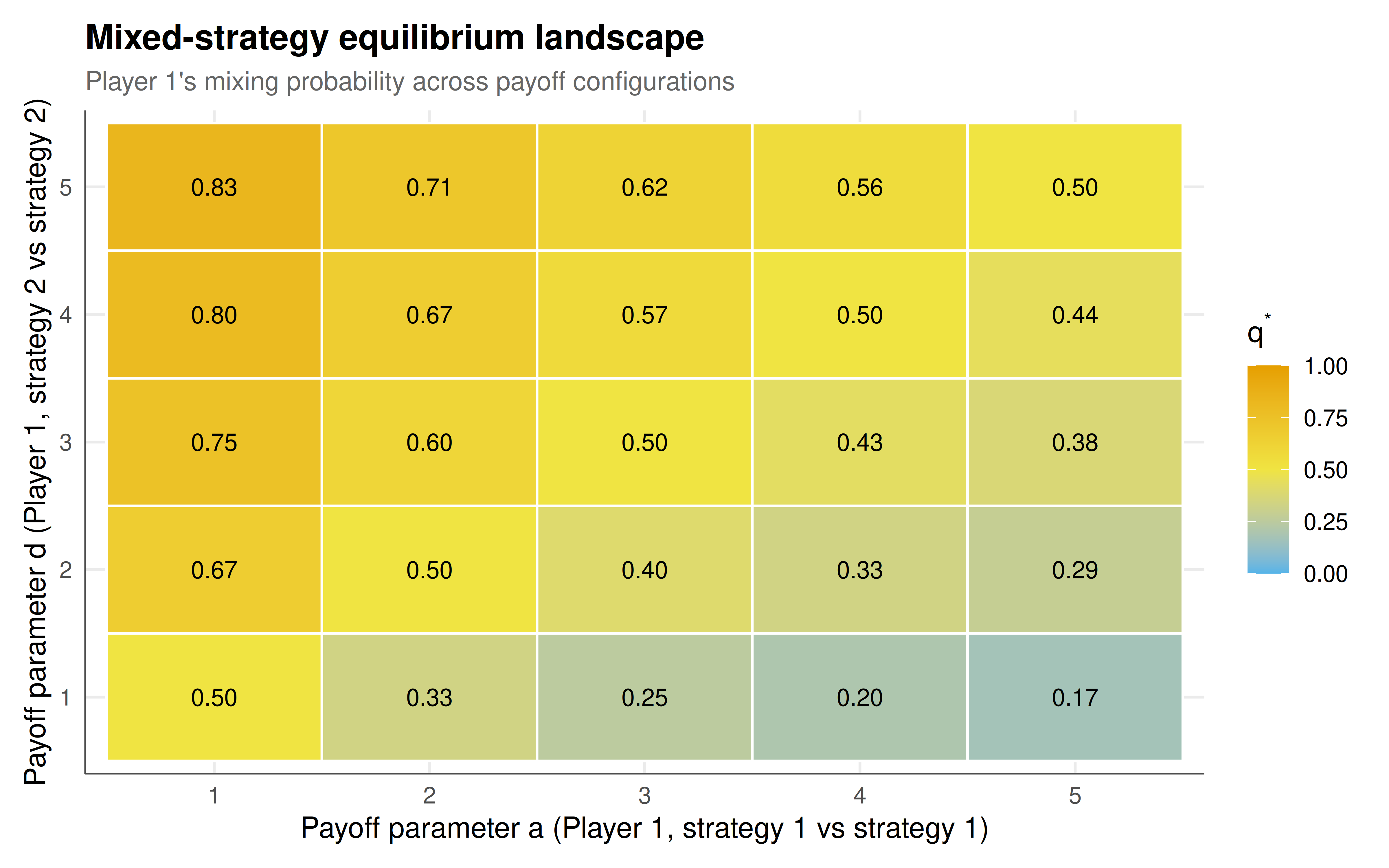
The static figure shows how the mixed-strategy Nash equilibrium probabilities vary across the payoff parameter space, forming an equilibrium landscape.
```{r}
#| label: fig-dashboard-static
#| fig-cap: "Figure 1. Mixed-strategy Nash equilibrium probabilities across payoff parameter space. Player 1's equilibrium mixing probability q* is shown as a heatmap over the (a, d) parameter grid, with contour lines indicating constant probability levels. Higher values of the diagonal payoffs shift the equilibrium toward more frequent play of the corresponding pure strategy. Okabe-Ito palette."
#| dev: [png, pdf]
#| fig-width: 8
#| fig-height: 5
#| dpi: 300
eq_data <- results |> filter(has_mixed)

p_static <- ggplot(eq_data, aes(x = factor(a), y = factor(d), fill = q_star)) +
  geom_tile(color = "white", linewidth = 0.5) +
  geom_text(aes(label = sprintf("%.2f", q_star)), size = 3.5, color = "black") +
  scale_fill_gradient2(
    low = okabe_ito[2], mid = okabe_ito[4], high = okabe_ito[1],
    midpoint = 0.5, limits = c(0, 1),
    name = expression(q^"*")
  ) +
  labs(
    title = "Mixed-strategy equilibrium landscape",
    subtitle = "Player 1's mixing probability across payoff configurations",
    x = "Payoff parameter a (Player 1, strategy 1 vs strategy 1)",
    y = "Payoff parameter d (Player 1, strategy 2 vs strategy 2)"
  ) +
  theme_publication() +
  theme(legend.position = "right")

p_static
```
## Interactive figure
The interactive version allows hovering over cells to inspect exact equilibrium values and parameter configurations.
```{r}
#| label: fig-dashboard-interactive
eq_interactive <- eq_data |>
  mutate(
    text = paste0(
      "a = ", a, ", d = ", d,
      "\np* = ", sprintf("%.3f", p_star),
      "\nq* = ", sprintf("%.3f", q_star)
    )
  )

p_int <- ggplot(eq_interactive, aes(x = factor(a), y = factor(d),
                                     fill = q_star, text = text)) +
  geom_tile(color = "white", linewidth = 0.5) +
  scale_fill_gradient2(
    low = okabe_ito[2], mid = okabe_ito[4], high = okabe_ito[1],
    midpoint = 0.5, limits = c(0, 1),
    name = "q*"
  ) +
  labs(
    title = "Interactive equilibrium explorer",
    x = "Payoff a", y = "Payoff d"
  ) +
  theme_publication() +
  theme(legend.position = "right")

ggplotly(p_int, tooltip = "text") |>
  config(displaylogo = FALSE,
         modeBarButtonsToRemove = c("select2d", "lasso2d"))
```
## Interpretation
The equilibrium landscape visualization reveals several important structural properties of parameterized games that would be difficult to appreciate from analytical expressions alone. The heatmap makes immediately visible the monotonic relationship between diagonal payoffs and equilibrium mixing probabilities: as Player 1's payoff from mutual cooperation (parameter $a$) increases relative to the mutual defection payoff (parameter $d$), the equilibrium probability of playing the first strategy shifts systematically. This visual monotonicity corresponds to the well-known comparative statics result that increasing a player's payoff from a particular outcome does not necessarily increase the probability of that outcome in the mixed equilibrium -- a counterintuitive finding that dashboards can effectively communicate.
The grid structure of the parameter exploration illustrates the dashboard design principle of systematic coverage. Rather than examining isolated parameter combinations, the grid ensures that the full parameter space is represented, revealing potential nonlinearities or threshold effects. In our specific example, the linear structure of the mixed-strategy formula produces a smoothly varying landscape, but more complex games -- such as those with three or more strategies, or games with constraints on strategy spaces -- can exhibit discontinuities, bifurcations, and regions where equilibria appear or disappear entirely.
From a practical dashboard design perspective, several lessons emerge. First, the choice of visual encoding matters: a heatmap with numeric labels provides both an overview (through color) and precise values (through text), satisfying the "overview first, zoom and filter, details on demand" mantra of information visualization. Second, the interactive version adds a layer of exploration without cluttering the display -- hovering reveals the full parameter configuration for any cell. Third, the coordinated display of both players' equilibrium probabilities (available in the tooltip) connects the two sides of the strategic interaction.
For deployment as a flexdashboard, this code would be wrapped in a layout specification with sidebar panels containing sliders for the fixed parameters ($b$, $c$, $e$, $f$, $g$, $h$), allowing users to explore how the equilibrium landscape reshapes when off-diagonal payoffs change. The reactive computation pattern -- parameter input, equilibrium solve, visualization update -- scales to more complex games. For Cournot oligopolies, the parameter space might include cost functions and demand elasticities; for auction models, bidder valuations and risk attitudes; for repeated games, discount factors and punishment strategies.
The dashboard approach also supports pedagogical objectives. Instructors can prepare specific parameter configurations that illustrate key concepts -- the disappearance of mixed equilibria when a game has dominant strategies, the convergence of mixed probabilities to corner solutions as one payoff dominates, or the symmetry of the equilibrium in symmetric games -- and guide students through a structured exploration.
## Extensions & related tutorials
The dashboard patterns demonstrated here connect to several other analytical approaches in the #equilibria collection. Extending the parameter grid to continuous spaces requires numerical optimization methods, while deploying the dashboard requires server infrastructure or alternative hosting solutions.
- [Agent-based modeling for game theory in R](../../simulations/agent-based-modeling-netlogo-style/)
- [Bootstrap methods for game-theoretic inference](../../statistical-foundations/bootstrap-methods-game-theory/)
- [Airbnb host pricing as a strategic game](../../real-world-data-applications/airbnb-pricing-strategy/)
- [Docker containers for reproducible game theory analysis](../../reproducibility-open-science/docker-reproducible-game-analysis/)
## References
::: {#refs}
:::