
Comparison families, adjusted p-values and plot annotations
Raban Heller
Source:vignettes/comparison-families.Rmd
comparison-families.Rmd

A study often reports several related comparisons. Whether their
p-values are adjusted, and over which set of hypotheses, is part of the
analysis and is decided in infercalcR. infereportR then shows the stored
raw or adjusted values and keeps the definition of the family attached
to every table, text and plot label. This vignette uses the
PlantGrowth and ToothGrowth data sets that
ship with R.
One result for a family of comparisons
PlantGrowth has three groups, which give three pairwise
comparisons. Each one is a Welch two-sample t-test computed by
infercalcR. The finished rows are then combined into a single result
with stable row identifiers and explicit contrast labels, so that the
family can be adjusted as a whole.
weight <- PlantGrowth$weight
group <- PlantGrowth$group
spec <- method_spec("t_means_two_independent_welch")

pairs <- data.frame(
  row_id = c("trt1-ctrl", "trt2-ctrl", "trt2-trt1"),
  comparison = c("trt1", "trt2", "trt2"),
  reference = c("ctrl", "ctrl", "trt1")
)

rows <- do.call(rbind, lapply(seq_len(nrow(pairs)), function(i) {
  fit <- run_inference(spec,
    x = weight[group == pairs$comparison[i]],
    y = weight[group == pairs$reference[i]])
  result_data(fit)
}))
rows$row_id <- pairs$row_id
rows$variable_id <- "weight"
rows$contrast <- paste(pairs$comparison, "minus", pairs$reference)

unadjusted <- new_inference_result(rows, list(
  method_id = "t_means_two_independent_welch",
  result_id = "plantgrowth-pairwise",
  population = "PlantGrowth: 30 plants, 10 per group"
))
The Holm adjustment is a calculation, so it also happens in infercalcR. It is applied once to the complete declared family:
family <- adjust_inference(unadjusted, method = "holm", family_id = "all-pairwise")Choose the stored p-value
The p argument selects which stored p-value is
displayed. Nothing is recalculated; the choice only decides which column
feeds p_display.
cols <- c("row_id", "contrast", "estimate_display", "p.value", "p.adjusted", "p_display")
report_table(family, p = "raw")[, cols]
#>      row_id        contrast estimate_display     p.value p.adjusted p_display
#> 1 trt1-ctrl trt1 minus ctrl           -0.371 0.250382509 0.25038251 p = 0.250
#> 2 trt2-ctrl trt2 minus ctrl            0.494 0.047899256 0.09579851 p = 0.048
#> 3 trt2-trt1 trt2 minus trt1            0.865 0.009298405 0.02789521 p = 0.009
report_table(family, p = "adjusted")[, cols]
#>      row_id        contrast estimate_display     p.value p.adjusted p_display
#> 1 trt1-ctrl trt1 minus ctrl           -0.371 0.250382509 0.25038251 p = 0.250
#> 2 trt2-ctrl trt2 minus ctrl            0.494 0.047899256 0.09579851 p = 0.096
#> 3 trt2-trt1 trt2 minus trt1            0.865 0.009298405 0.02789521 p = 0.028
Asking for adjusted values that were never computed is an error rather than a silent fallback to raw p-values:
try(report_table(unadjusted, p = "adjusted"))
#> Error : requested adjusted p-values are unavailable for one or more selected rows
Select rows after adjustment
rows picks rows for display. Selecting happens after the
adjustment, and the metadata still describes the full family, including
its size and members:
one <- report_table(family, rows = "trt2-trt1", p = "adjusted")
one[, cols]
#>      row_id        contrast estimate_display     p.value p.adjusted p_display
#> 1 trt2-trt1 trt2 minus trt1            0.865 0.009298405 0.02789521 p = 0.028
str(report_metadata(one)$adjustment)
#> List of 1
#>  $ :List of 5
#>   ..$ family_id          : chr "all-pairwise"
#>   ..$ rows               : chr [1:3] "trt1-ctrl" "trt2-ctrl" "trt2-trt1"
#>   ..$ size               : int 3
#>   ..$ method             : chr "holm"
#>   ..$ interval_adjustment: chr "unchanged"
Full text names the adjustment method next to the displayed p-value:
cat(report_text(family, p = "adjusted"), sep = "\n")
#> t_means_two_independent_welch; mean difference (x minus reference or y); trt1 minus ctrl: estimate -0.371; 95% interval [-1.03, 0.288] (Welch t; identity; pointwise); statistic -1.19; p = 0.250 (adjusted); recorded adjustment: holm; n = 20; excluded = 0.
#> t_means_two_independent_welch; mean difference (x minus reference or y); trt2 minus ctrl: estimate 0.494; 95% interval [0.00513, 0.983] (Welch t; identity; pointwise); statistic 2.13; p = 0.096 (adjusted); recorded adjustment: holm; n = 20; excluded = 0.
#> t_means_two_independent_welch; mean difference (x minus reference or y); trt2 minus trt1: estimate 0.865; 95% interval [0.249, 1.48] (Welch t; identity; pointwise); statistic 3.01; p = 0.028 (adjusted); recorded adjustment: holm; n = 20; excluded = 0.
Stars and unavailable results
The stars preset uses the thresholds 0.05, 0.01, 0.001
and 0.0001:
stars <- report_text(family, p = "adjusted", style = "stars")
data.frame(row_id = names(stars), label = as.character(stars))
#>      row_id label
#> 1 trt1-ctrl    ns
#> 2 trt2-ctrl    ns
#> 3 trt2-trt1     *
A result that could not be computed keeps its status. It never
receives stars or ns, and full text states the recorded
reason:
incomplete <- new_inference_result(
  data.frame(
    row_id = c("a", "b"), estimand = "mean difference",
    estimate = c(0.8, NA), conf.low = c(0.1, NA), conf.high = c(1.5, NA),
    conf.level = 0.95, p.value = c(0.03, NA), status = c("ok", "undefined"),
    reason = c(NA, "fewer than two observations in one group")
  ),
  list(method_id = "example", result_id = "incomplete")
)
cat(report_text(incomplete, style = "stars"), sep = "\n")
#> *
#> unavailable (undefined)
cat(report_text(incomplete), sep = "\n")
#> example; mean difference: estimate 0.8; 95% interval [0.1, 1.5]; p = 0.030 (reported).
#> example; mean difference; p unavailable (reported); status undefined (fewer than two observations in one group).
Brackets on a plot
The remaining sections need the optional ggplot2 package; their chunks run only when it is installed.
Each bracket is described by one row of a positions data frame.
Coordinates are in data units. group1 and
group2 name the endpoints, and groups gives
the order of the groups on the discrete axis.
library(ggplot2)

positions <- data.frame(
  row_id = pairs$row_id,
  group1 = pairs$reference,
  group2 = pairs$comparison,
  y_position = c(6.5, 7.3, 6.9)
)

base <- ggplot(PlantGrowth, aes(group, weight)) +
  geom_boxplot(width = 0.5) +
  labs(x = NULL, y = "Dried weight")

base + stat_inference(family, positions, groups = levels(group),
  p = "adjusted", tip_length = 0.1)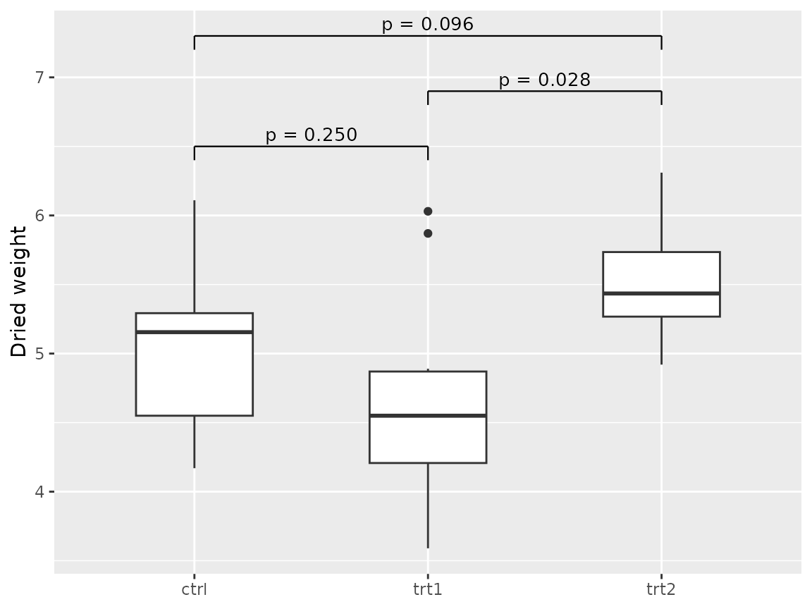
Changing the order of the axis moves the brackets but never reverses
a contrast. Below, trt2 is drawn first, and each label
still shows the stored difference with its original sign, for example
trt2 minus trt1:
reordered <- PlantGrowth
reordered$group <- factor(reordered$group, levels = c("trt2", "trt1", "ctrl"))

ggplot(reordered, aes(group, weight)) +
  geom_boxplot(width = 0.5) +
  stat_inference(family, positions, groups = levels(reordered$group),
    label = "estimate_ci", tip_length = 0.1) +
  labs(x = NULL, y = "Dried weight")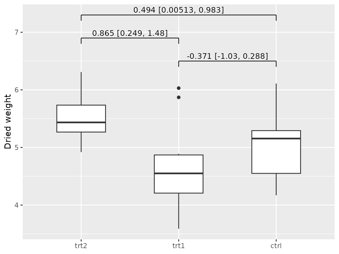
Text labels for omnibus tests
An omnibus test has no pair of endpoints, so it is annotated with
text only. Its position gives x and y_position
instead of group1 and group2:
omnibus <- run_inference(method_spec("anova_one_way_welch"),
  x = weight, group = group, result_id = "welch-anova")
report_table(omnibus)[, c("component", "estimand", "statistic_display", "p_display")]
#>   component                                                 estimand
#> 1   omnibus One-way analysis of means (not assuming equal variances)
#>   statistic_display p_display
#> 1              5.18 p = 0.017
pairwise_plot <- base + stat_inference(family, positions, groups = levels(group),
  p = "adjusted", tip_length = 0.1)
text_position <- data.frame(row_id = result_data(omnibus)$row_id,
  x = 2, y_position = 7.7)
annotate_inference(pairwise_plot, omnibus, text_position,
  template = "Welch ANOVA: {p}")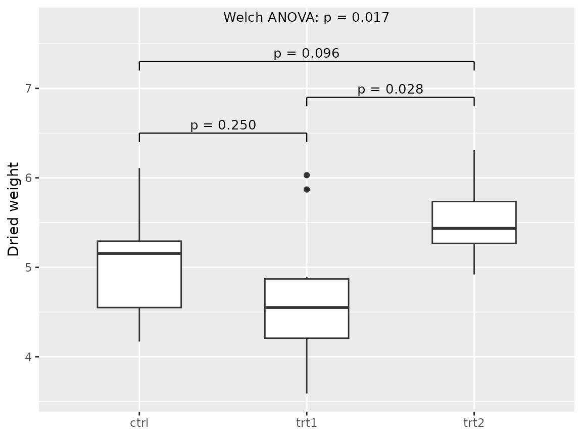
annotate_inference() adds the same layers as
stat_inference() but first checks that the existing plot
uses Cartesian coordinates or coord_flip(). Polar and other
nonlinear coordinates are rejected.
Flipped coordinates and transformed scales
Positions are always given in the original data units. With
scale_y_log10(), a y_position of 100 is drawn
at 2 on the log scale, transformed exactly once. For horizontal plots,
adjust the text justification and leave room for the labels:
pairwise_flipped <- base +
  stat_inference(family, positions, groups = levels(group), p = "adjusted",
    tip_length = 0.1, text_hjust = -0.1, text_vjust = 0.5) +
  scale_y_continuous(expand = expansion(mult = c(0.05, 0.25))) +
  coord_flip()
pairwise_flipped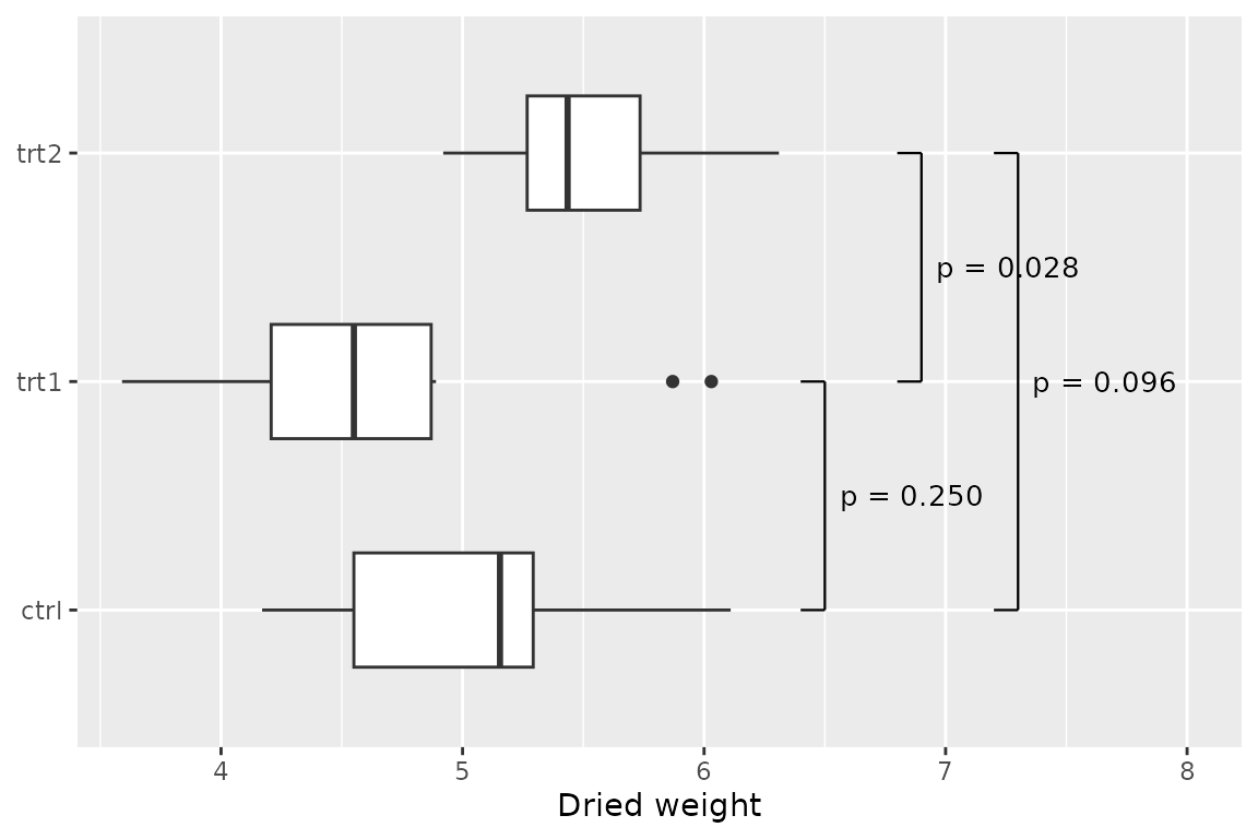
Results per facet
Results that belong to subgroups carry their subgroup key as a
column, and the result metadata declares it in facet_vars.
Here the two supplements in ToothGrowth are compared
separately at each dose:
tg <- ToothGrowth
doses <- sort(unique(tg$dose))
by_dose <- do.call(rbind, lapply(doses, function(d) {
  fit <- run_inference(spec,
    x = tg$len[tg$dose == d & tg$supp == "OJ"],
    y = tg$len[tg$dose == d & tg$supp == "VC"])
  out <- result_data(fit)
  out$dose <- d
  out
}))
by_dose$row_id <- paste0("OJ-VC-dose-", doses)
by_dose$contrast <- "OJ minus VC"

dose_results <- new_inference_result(by_dose, list(
  method_id = "t_means_two_independent_welch",
  result_id = "toothgrowth-by-dose",
  population = "ToothGrowth: 10 animals per supplement and dose",
  facet_vars = "dose"
))
report_table(dose_results)[, c("row_id", "dose", "estimate_display", "p_display")]
#>           row_id dose estimate_display p_display
#> 1 OJ-VC-dose-0.5  0.5             5.25 p = 0.006
#> 2   OJ-VC-dose-1  1.0             5.93 p = 0.001
#> 3   OJ-VC-dose-2  2.0            -0.08 p = 0.964
These three p-values are not adjusted. The positions repeat the facet key, and it must match the stored rows exactly; a missing or conflicting key is an error instead of a label copied into every panel:
facet_positions <- data.frame(
  row_id = by_dose$row_id, dose = doses,
  group1 = "OJ", group2 = "VC",
  y_position = c(24, 30, 36)
)

ggplot(tg, aes(supp, len)) +
  geom_boxplot(width = 0.5) +
  facet_wrap(~dose) +
  stat_inference(dose_results, facet_positions, groups = levels(tg$supp),
    tip_length = 1) +
  labs(x = "Supplement", y = "Odontoblast length")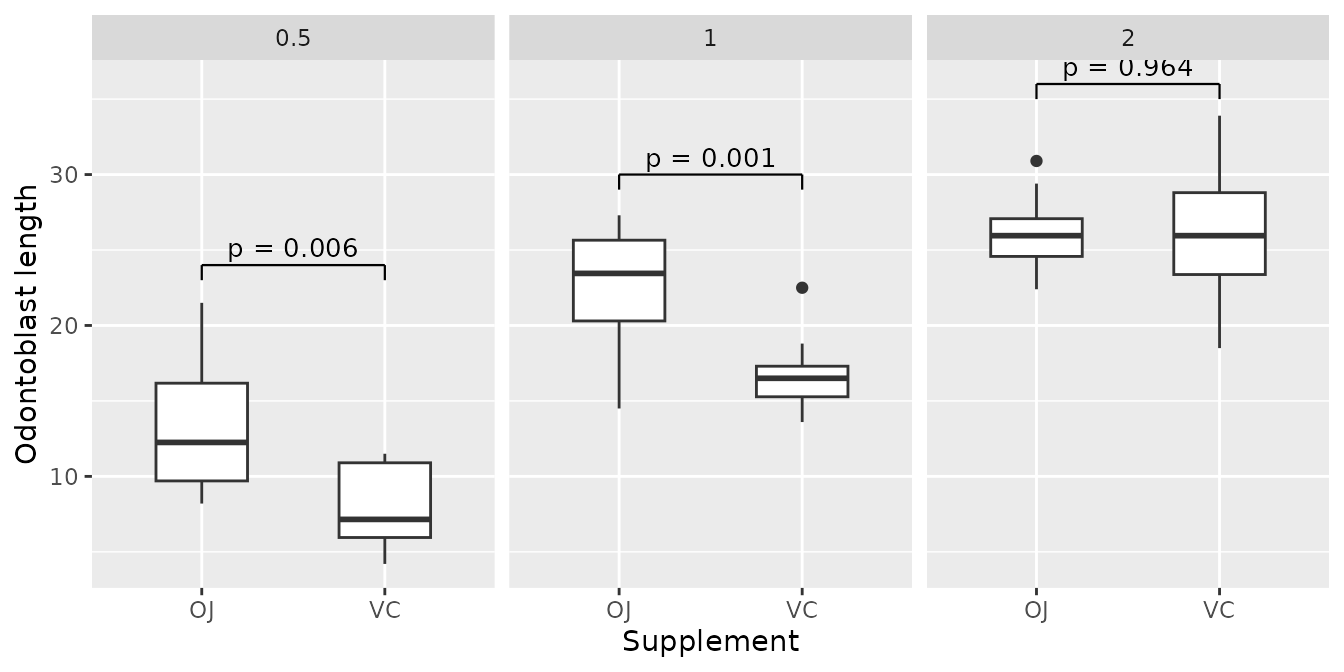
Annotations are placed only where the positions say. Automatic
placement, automatic dodging and free facet scales are not inferred. For
dodged groups, give numeric xmin and xmax
instead of group1 and group2.
Acknowledgments and sources
This package is part of an inference suite (infercalcR, inferguidR and infereportR) that is deeply inspired by DescrTab2 [1], developed at the Institute of Medical Biometry (IMBI), Heidelberg University, by Jan Meis, Lukas Baumann, Maximilian Pilz and Lukas Sauer. Its test-choice tree, its validation statement and its practice of computing each test with an established implementation are the model for how the suite chooses, computes and reports statistical tests. DescrTab2 was archived on CRAN on 18 October 2025; its source code remains available on GitHub. The methods-consulting pages of the University of Zurich [2], with their decision tree, decision assistant, worked examples and explanations, inspired the guidance in the suite. Power and sample-size planning and the distribution calculator follow G*Power 3.1 [3, 4]. We thank the authors of these works for making them openly available. The package README cites all software the package uses.
- Meis J, Baumann L, Pilz M, Sauer L (2022). DescrTab2: Publication Quality Descriptive Statistics Tables. R package version 2.1.16. https://doi.org/10.32614/CRAN.package.DescrTab2. Source code, including the development version 2.1.26: https://github.com/imbi-heidelberg/DescrTab2.
- Universität Zürich, Methodenberatung. Datenanalyse mit SPSS: decision tree (Entscheidbaum), decision assistant (Entscheidassistent) and method pages with examples and explanations. https://www.methodenberatung.uzh.ch/de/datenanalyse_spss.html. Accessed 3 October 2026.
- Faul F, Erdfelder E, Lang A-G, Buchner A (2007). G*Power 3: A flexible statistical power analysis program for the social, behavioral, and biomedical sciences. Behavior Research Methods, 39(2), 175-191. https://doi.org/10.3758/BF03193146.
- Faul F, Erdfelder E, Buchner A, Lang A-G (2009). Statistical power analyses using G*Power 3.1: Tests for correlation and regression analyses. Behavior Research Methods, 41(4), 1149-1160. https://doi.org/10.3758/BRM.41.4.1149.