
Getting started with infereportR
Raban Heller
Source:vignettes/getting-started.Rmd
getting-started.Rmd

infereportR presents statistical results that are already finished.
It turns them into tables, sentences for a manuscript and labels for a
plot. It does not run tests, fit models, compute intervals or adjust
p-values. Those steps belong to infercalcR, which stores every result in
a common, plain-data format. infereportR reads that format through
infercalcR::result_data() and
infercalcR::result_metadata() and formats what it
finds.
This vignette walks through one result from calculation to table,
text and plot. It uses the PlantGrowth data set that ships
with R and runs offline.
Compute a result with infercalcR
PlantGrowth holds the dried weight of 30 plants: 10 in a
control condition (ctrl) and 10 in each of two treatment
conditions (trt1, trt2). The analysis is
chosen in advance: a Welch two-sample t-test comparing trt2
with ctrl. The method, sidedness and confidence level are
fixed in the specification before any data are seen.
trt2 <- PlantGrowth$weight[PlantGrowth$group == "trt2"]
ctrl <- PlantGrowth$weight[PlantGrowth$group == "ctrl"]

welch <- run_inference(
  method_spec("t_means_two_independent_welch"),
  x = trt2, y = ctrl,
  result_id = "trt2-vs-ctrl"
)
welch
#> <inference> t_means_two_independent_welch
#>                           row_id                                 estimand
#>  t_means_two_independent_welch:1 mean difference (x minus reference or y)
#>  estimate p.reported status
#>     0.494 0.04789926     ok
The estimate is the difference in means, x minus
y, here trt2 minus ctrl. All
numbers are now final. Every step below only reads them.
Report a table
report_table() returns an ordinary data frame with one
row per stored result row. The analytical columns keep their full
precision:
tab <- report_table(welch)
tab[, c("estimand", "estimate", "conf.low", "conf.high", "p.value", "n")]
#>                                   estimand estimate   conf.low conf.high
#> 1 mean difference (x minus reference or y)    0.494 0.00512787 0.9828721
#>      p.value  n
#> 1 0.04789926 20
Formatted values sit in separate columns ending in
_display, so rounding never replaces a stored number:
tab[, c("estimate_display", "interval_display", "p_display", "confidence_display")]
#>   estimate_display interval_display p_display confidence_display
#> 1            0.494 [0.00513, 0.983] p = 0.048                95%
p_selected and p_selection record which
stored p-value is shown. The default is the reported p-value;
p = "raw" and p = "adjusted" select the other
stored columns. The number of digits and the decimal mark change the
presentation only:
report_table(welch, digits = 2, p_digits = 4, decimal_mark = ",")[
  , c("estimate_display", "interval_display", "p_display")]
#>   estimate_display interval_display  p_display
#> 1             0,49   [0,0051, 0,98] p = 0,0479
Because the result is a plain data frame, any table tool can print
it. For example, with knitr::kable():
knitr::kable(
  tab[, c("estimand", "estimate_display", "interval_display", "p_display", "n")],
  col.names = c("Estimand", "Estimate", "Interval", "p-value", "n")
)| Estimand | Estimate | Interval | p-value | n |
|---|---|---|---|---|
| mean difference (x minus reference or y) | 0.494 | [0.00513, 0.983] | p = 0.048 | 20 |
Report text
report_text() writes one neutral sentence per row. The
full style names the method, the estimand, the estimate, the interval
with its confidence level and method, the test statistic, the p-value
together with which p-value it is, the sample size and the number of
excluded observations:
cat(report_text(welch), sep = "\n")
#> t_means_two_independent_welch; mean difference (x minus reference or y): estimate 0.494; 95% interval [0.00513, 0.983] (Welch t; identity; pointwise); statistic 2.13; p = 0.048 (reported); n = 20; excluded = 0.
The sentence contains no interpretation. It does not call a result significant or relevant; that judgment stays with the author.
Shorter presets suit tables and figure legends:
cat(report_text(welch, style = "estimate_ci_p"), sep = "\n")
#> 0.494 [0.00513, 0.983]; p = 0.048
cat(report_text(welch, style = "p"), sep = "\n")
#> p = 0.048
A template inserts stored fields into your own wording. The supported
fields are estimate, ci, p,
statistic, method, estimand,
contrast, status and n. Templates
are substituted, never evaluated, and an unknown field is an error:
cat(report_text(welch,
  template = "trt2 minus ctrl: {estimate} {ci}; {p}; n = {n}"), sep = "\n")
#> trt2 minus ctrl: 0.494 [0.00513, 0.983]; p = 0.048; n = 20
try(report_text(welch, template = "{mean}"))
#> Error : template contains an unsupported field or malformed braces
Annotate a plot
The optional ggplot2 integration draws brackets and labels from the same stored result. The chunks in this section run only when ggplot2 is installed.
A positions data frame states where each annotation goes. It has one
row per result row, identified by row_id, and a
y_position in data units. Named endpoints
(group1, group2) need the order of the groups
on the discrete axis, given in groups.
library(ggplot2)

positions <- data.frame(
  row_id = result_data(welch)$row_id,
  group1 = "ctrl", group2 = "trt2",
  y_position = 6.6
)

ggplot(PlantGrowth, aes(group, weight)) +
  geom_boxplot(width = 0.5) +
  stat_inference(welch, positions, groups = levels(PlantGrowth$group),
    label = "estimate_ci_p", tip_length = 0.1) +
  labs(x = NULL, y = "Dried weight")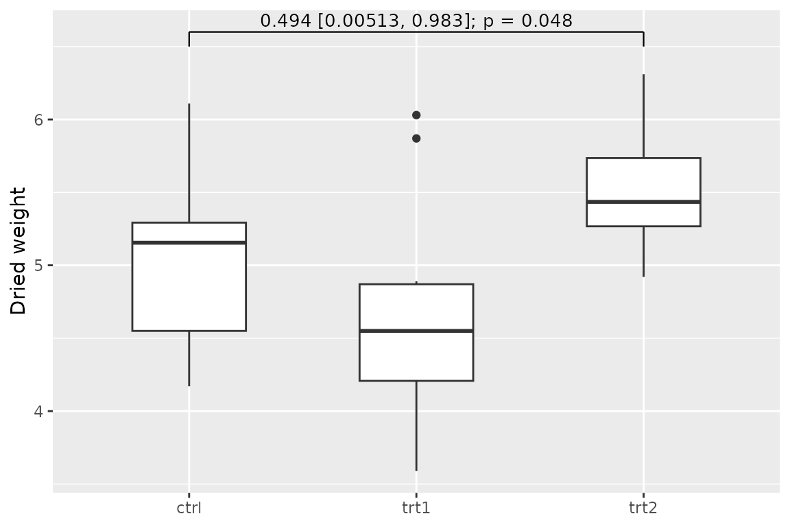
stat_inference() returns ordinary ggplot2 layers. No
test runs while the plot is built or drawn, and the label is the same
text that report_text() gives for
style = "estimate_ci_p". tip_length is also in
data units.
Keep the provenance
Tables and text carry the result metadata as an attribute.
report_metadata() retrieves it, for example to record the
method, the result identifier and the analysis population next to a
table:
meta <- report_metadata(tab)
meta[c("method_id", "result_id", "kind")]
#> $method_id
#> [1] "t_means_two_independent_welch"
#>
#> $result_id
#> [1] "trt2-vs-ctrl"
#>
#> $kind
#> [1] "inference"
str(meta$population)
#> List of 3
#>  $ n_input   : int 20
#>  $ n_used    : num 20
#>  $ n_excluded: num 0
Shared formatters
Tables, text and plot labels use the same three formatters, which are also exported:
format_estimate(c(0.494, -1.23456, NA))
#> [1] "0.494"       "-1.23"       "unavailable"
format_interval(c(0.00513, -Inf), c(0.983, 2))
#> [1] "[0.00513, 0.983]" "[-Inf, 2]"
format_p(c(0.0479, 0.0004, 0, NA))
#> [1] "p = 0.048"     "p < 0.001"     "p < 0.001"     "p unavailable"
A p-value below the display threshold, including a stored zero, is
shown as p < 0.001 rather than p = 0. A
missing p-value is shown as unavailable and never as nonsignificant.
Infinite interval limits stay infinite.
Next steps
-
vignette("comparison-families", package = "infereportR")combines several comparisons, displays adjusted p-values and covers plot annotations in more detail. -
vignette("descriptive-tables", package = "infereportR")describes data with explicit denominators and joins supplied inference.
Acknowledgments and sources
This package is part of an inference suite (infercalcR, inferguidR and infereportR) that is deeply inspired by DescrTab2 [1], developed at the Institute of Medical Biometry (IMBI), Heidelberg University, by Jan Meis, Lukas Baumann, Maximilian Pilz and Lukas Sauer. Its test-choice tree, its validation statement and its practice of computing each test with an established implementation are the model for how the suite chooses, computes and reports statistical tests. DescrTab2 was archived on CRAN on 18 October 2025; its source code remains available on GitHub. The methods-consulting pages of the University of Zurich [2], with their decision tree, decision assistant, worked examples and explanations, inspired the guidance in the suite. Power and sample-size planning and the distribution calculator follow G*Power 3.1 [3, 4]. We thank the authors of these works for making them openly available. The package README cites all software the package uses.
- Meis J, Baumann L, Pilz M, Sauer L (2022). DescrTab2: Publication Quality Descriptive Statistics Tables. R package version 2.1.16. https://doi.org/10.32614/CRAN.package.DescrTab2. Source code, including the development version 2.1.26: https://github.com/imbi-heidelberg/DescrTab2.
- Universität Zürich, Methodenberatung. Datenanalyse mit SPSS: decision tree (Entscheidbaum), decision assistant (Entscheidassistent) and method pages with examples and explanations. https://www.methodenberatung.uzh.ch/de/datenanalyse_spss.html. Accessed 3 October 2026.
- Faul F, Erdfelder E, Lang A-G, Buchner A (2007). G*Power 3: A flexible statistical power analysis program for the social, behavioral, and biomedical sciences. Behavior Research Methods, 39(2), 175-191. https://doi.org/10.3758/BF03193146.
- Faul F, Erdfelder E, Buchner A, Lang A-G (2009). Statistical power analyses using G*Power 3.1: Tests for correlation and regression analyses. Behavior Research Methods, 41(4), 1149-1160. https://doi.org/10.3758/BRM.41.4.1149.