![]()
![]()
![]()
![]()
![]()
Load data
sim <- load_example_data()
print(sim)
#>
#> ── dynasimR_data ───────────────────────────────────────────────────────────────
#> • Scenarios: 4
#> • Profile: "Profile_A"
#> • Summary rows: 200
#> • Entity events: 16000
#> • Loaded: "2026-06-24 09:25"
#> • Path: /home/runner/work/_temp/Library/dynasimR/extdata
Time-to-event analysis
km <- km_estimate(sim, endpoint = "stage2",
                  stratify_by = "scenario")
plot_km(km, title = "Time-to-stage-2")
#> Warning: Removed 2 rows containing missing values or values outside the scale range
#> (`geom_ribbon()`).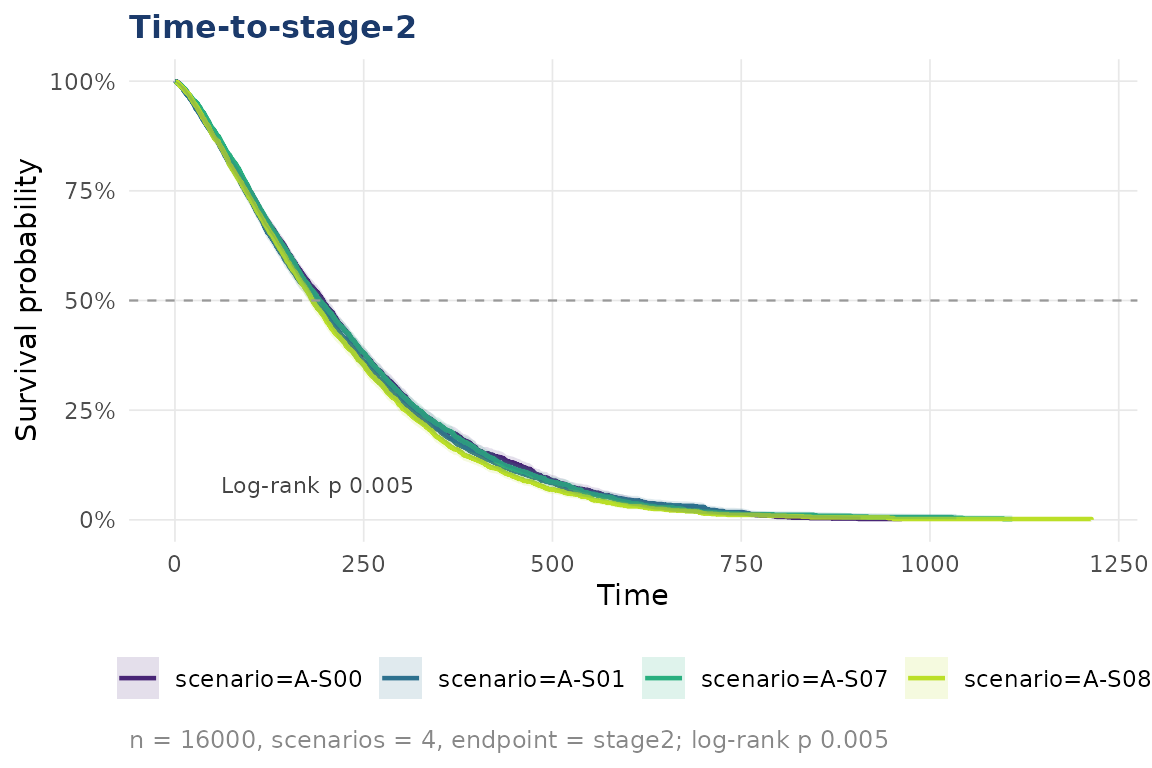
Policy effect
pol <- policy_effect(sim,
  policy_a_scenario = "A-S08",
  policy_b_scenario = "A-S07",
  n_bootstrap       = 200)
cat(pol$narrative)
#> Under policy A (scenario A-S08), an event-rate reduction of 7.4 percentage points (95\%-CI: -9 to -5.6) was observed versus policy B (scenario A-S07) (Wilcoxon test: W = 215, p < 0.001). The Compliance Index was higher under policy A (0.919 vs. 0.658).
Autonomy trade-off
Only two AL points are present in the shipped example data, but the machinery is the same for a full AL sweep.
al <- al_efficiency(
  sim,
  al_scenarios         = c("0" = "A-S00", "1" = "A-S01"),
  compliance_threshold = 0.80,
  n_bootstrap          = 200
)
plot_al_tradeoff(al)
#> `height` was translated to `width`.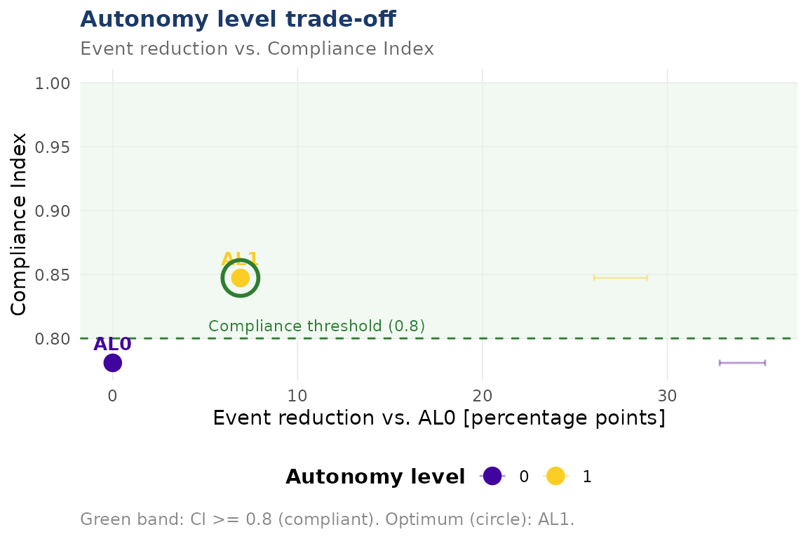
Manuscript-ready export
export_latex_table(
  data     = pol$effect_sizes,
  filename = "policy_table.tex",
  caption  = "Policy effect sizes.",
  label    = "policy"
)
Launching the dashboard
launch_app()                                        # example data
launch_app(data_dir = "~/my-simulation/data/raw")
Use of LLM tools
Portions of this package were prepared with assistance from large
language model tooling for narrowly defined, non-authorial tasks:
copyediting, prose smoothing, Markdown/LaTeX formatting, scaffolding of
boilerplate files (CI configs, build scripts), code refactoring. The
tools used were Chat AI,
the LLM service of KISSKI (GWDG), and a self-hosted Mistral
Small (24B, Apache-2.0) run locally via Ollama and the ollamar R
package — local inference only, with no data sent to third parties for
the self-hosted model.
All scientific claims, methodological choices, analyses, interpretations, and conclusions are the author’s own. No LLM-generated text was incorporated without review and revision, and every reference was verified against its DOI, arXiv ID, or ISBN.