Figures and tables

Every panel of the zhncommandR dashboard is a thin wrapper around an exported function, so the exact figures and tables you see in the app can be reproduced in a script or report. This vignette walks through them on the bundled, 100 % synthetic example cohort.

The tables behind the panels

The three readers turn the tumour-documentation sheets into tidy data frames (cleaned column names, derived treatment year):

cohort <- zhn_read_cohort(path, verbose = FALSE)
cohort |>
  dplyr::count(diagnose, name = "Faelle", sort = TRUE) |>
  dplyr::slice_head(n = 6) |>
  knitr::kable(caption = "Cohort by entity (top 6)")

Cohort by entity (top 6)

diagnose	Faelle
Mantelzell-Lymphom	15
MDS	14
Multiples Myelom	14
AML	10
CLL	10
DLBCL	9

The S3 wrappers print and summarise themselves — a one-line cohort overview:

summary(cohort)
#>   rows columns diagnoses years_covered sheet_to_use
#> 1  100      31        10             4   Basisdaten

OPS-8-544 therapy blocks

therapy <- zhn_read_therapy(path, verbose = FALSE)
blocks  <- zhn_prepare_therapy_blocks(therapy)
blocks |>
  dplyr::count(therapieprotokoll, name = "Bloecke", sort = TRUE) |>
  dplyr::slice_head(n = 6) |>
  knitr::kable(caption = "Complex-chemotherapy blocks per protocol (top 6)")

Complex-chemotherapy blocks per protocol (top 6)

therapieprotokoll	Bloecke
Azacitidin	106
ABVD	105
DA-EPOCH-R	105
AraC	95
Rd	92
7+3	88

summary(blocks)
#>   blocks patients protocols diagnoses
#> 1   1000      100        11        10

OPS-1-941 complex diagnostics

diag    <- zhn_read_diagnostics(path, verbose = FALSE)
dblocks <- zhn_prepare_diagnostic_blocks(diag)
summary(dblocks)
#>   cases patients diagnoses
#> 1   130       75        10
#>                                                          components
#> 1 morphologie, immunphanotypisierung, zytogenetik, molekulargenetik

Oncoprint and cytogenetics

The alteration free-text is split and classified into a tidy long table; only true mutations/variants go to the oncoprint, structural/cytogenetic findings are tabulated separately.

onco <- zhn_parse_oncoprint(cohort)
onco |>
  dplyr::count(alteration_class, name = "n", sort = TRUE) |>
  knitr::kable(caption = "Oncoprint alterations by class")

Oncoprint alterations by class

alteration_class	n
Mutation/Variante	81
Strukturell/Zytogenetik: Deletion/Loss	34

cyto <- zhn_parse_cytogenetics(cohort)
cyto |>
  dplyr::count(alteration_class, name = "n", sort = TRUE) |>
  knitr::kable(caption = "Cytogenetic findings by class")

Cytogenetic findings by class

alteration_class	n
Strukturell/Zytogenetik: Translokation/Rearrangement/Bruch	45
Strukturell/Zytogenetik: Deletion/Loss	42
Strukturell/Zytogenetik: Zugewinn/Amplifikation	35
Strukturell/Zytogenetik: Komplexer Karyotyp	16
Mutation/Variante	8

The figures

All figures share one theme (zhn_theme()) in the Hugo Coder look — a single blue data-ink accent (zhn_pal$accent), Inter type and a minimal panel — and each is a plain ggplot object you can extend.

zhn_plot_diagnoses(cohort, col = "diagnose")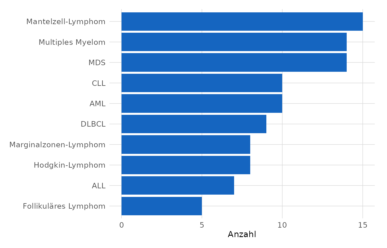

zhn_plot_cases_by_year(cohort)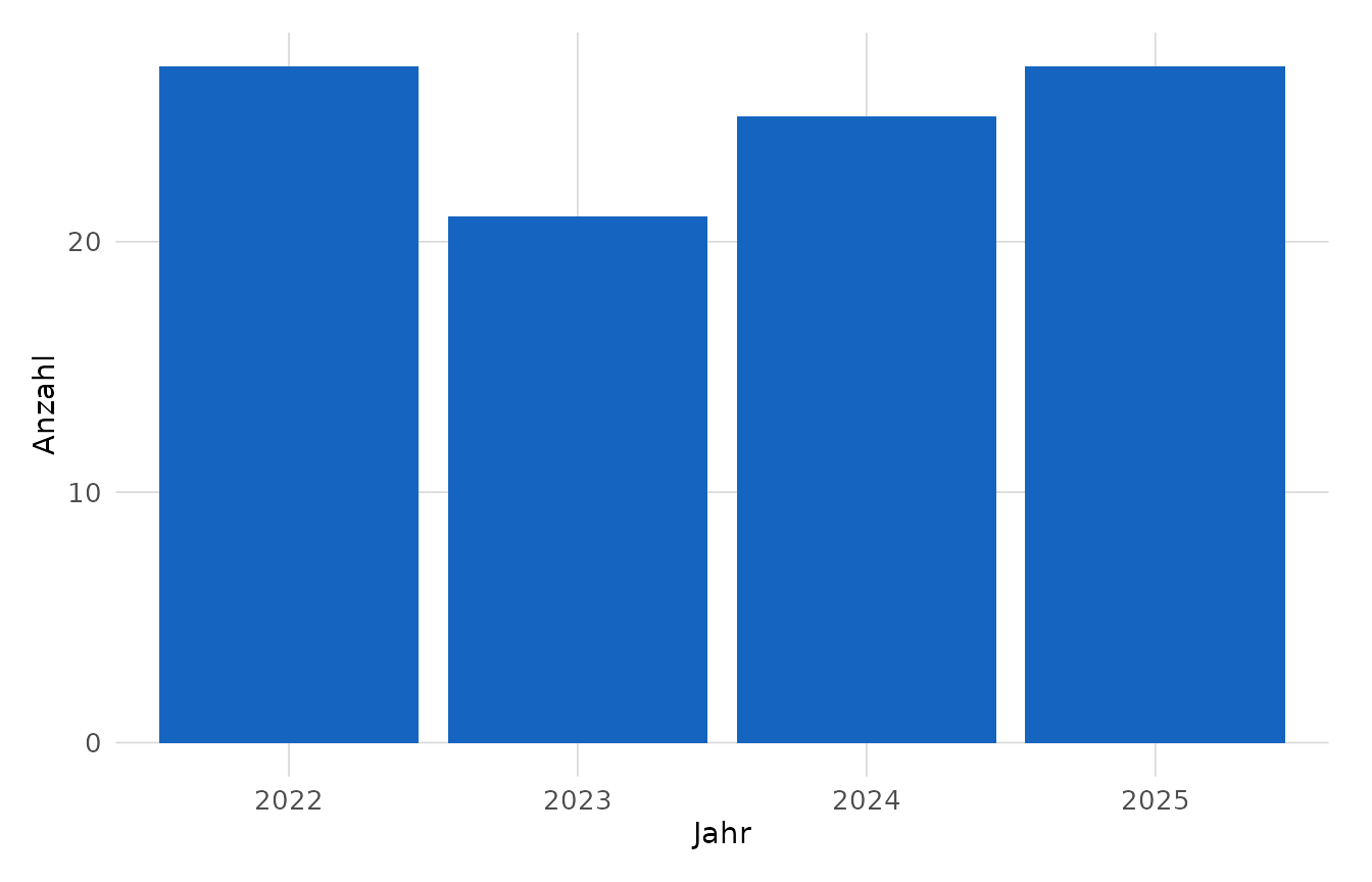

A publication-ready Kaplan-Meier curve (overall survival) with confidence interval, censoring marks and a numbers-at-risk table:

zhn_plot_km(cohort, time_col = "os", event_col = "death_event",
            title = "Gesamtüberleben (synthetisch)")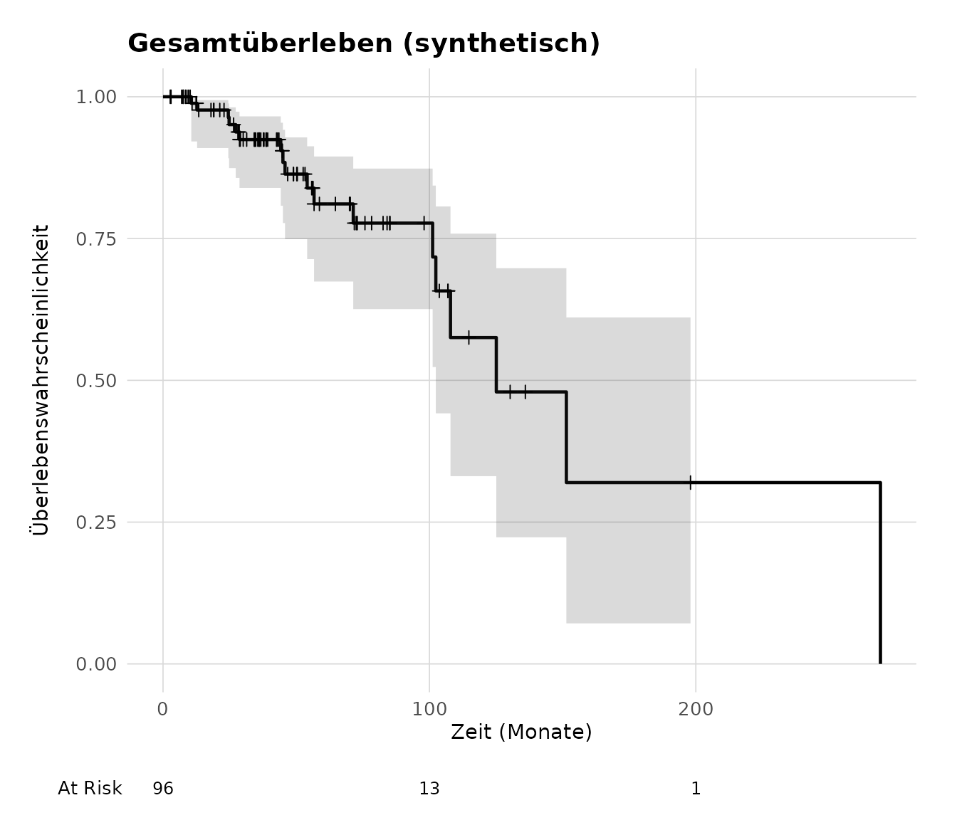

See vignette("zhncommandR") for the full set of Kaplan-Meier options (grouping, log-rank p, Cox hazard ratio with proportional-hazards check, pairwise comparisons, cumulative-incidence scale).

Exporting paper-ready files

zhn_save_plot() writes any of these figures at 600 dpi (PNG, via ragg) or as a vector PDF (via cairo_pdf, with the Inter font embedded). The transparency toggle from the app maps to the transparent argument.

p <- zhn_plot_cases_by_year(cohort)
zhn_save_plot(p, "cases_by_year.png", format = "png", width = 8, height = 5)
zhn_save_plot(p, "cases_by_year.pdf", format = "pdf", transparent = TRUE)