Getting started with zhncommandR • zhncommandR

zhncommandR packages the ZHN Auditor dashboard — a Shiny app for live evaluation of haematological tumour-centre cohorts — together with the backend helpers that drive it. The dashboard is launched with zhn_run_app(). The rest of this vignette shows the same analyses run programmatically against the bundled synthetic example.

This package ships three vignettes:

Getting started (this one) — readers, parsers and a first survival curve.
Figures and tables — the publication-ready figures and the tables behind every dashboard panel, run programmatically.
The Shiny dashboard — a guided tour of the interactive auditor app.

Example data

The package ships a 100 % synthetic example workbook with three sheets: Basisdaten, Komplexe Chemotherapie, Komplexe Diagnostik.

path <- zhn_example_path()
basename(path)
#> [1] "zhn_example.xlsx"

Reading the cohort

cohort <- zhn_read_cohort(path, verbose = FALSE)
cohort |>
  dplyr::select(dplyr::any_of(c(
    "name", "diagnose", "behandlungsjahr", "primaerfall",
    "psychoonkologie", "pfs", "os"
  ))) |>
  dplyr::glimpse()
#> Rows: 100
#> Columns: 7
#> $ name            <chr> "Muster, Fall 001", "Muster, Fall 002", "Muster, Fall …
#> $ diagnose        <chr> "Marginalzonen-Lymphom", "DLBCL", "Multiples Myelom", …
#> $ behandlungsjahr <int> 2024, 2024, 2025, 2022, 2024, 2022, 2023, 2023, 2025, …
#> $ primaerfall     <chr> "nein", "ja", "ja", "nein", "ja", "ja", "ja", "nein", …
#> $ psychoonkologie <chr> "nein", "ja", "nein", "nein", "nein", "nein", "nein", …
#> $ pfs             <dbl> 8.0, 23.4, 26.4, 49.1, 26.5, 5.3, 20.7, 10.8, 1.0, 4.3…
#> $ os              <dbl> 45.8, 72.5, 82.6, 50.4, 56.7, 12.4, 54.1, 13.4, 3.0, 1…

zhn_read_cohort() calls janitor::clean_names(), drops empty none* columns, and derives behandlungsjahr from the first matching date column.

Quality indicators

The indicator table on the dashboard is just a dplyr summary of a fixed indicator list:

indicators <- c("tumorkonferenz", "psychoonkologie", "sozialdienst",
                "hiv_hepatitis")

cohort |>
  dplyr::select(dplyr::any_of(indicators)) |>
  tidyr::pivot_longer(
    dplyr::everything(),
    names_to = "Indikator", values_to = "Wert"
  ) |>
  dplyr::group_by(Indikator) |>
  dplyr::summarise(
    Positiv = sum(zhncommandR:::.as_yesno(Wert) %in% TRUE, na.rm = TRUE),
    Gesamt  = dplyr::n(),
    Anteil  = round(Positiv / Gesamt, 2),
    .groups = "drop"
  )
#> # A tibble: 4 × 4
#>   Indikator       Positiv Gesamt Anteil
#>   <chr>             <int>  <int>  <dbl>
#> 1 hiv_hepatitis        93    100   0.93
#> 2 psychoonkologie      53    100   0.53
#> 3 sozialdienst         43    100   0.43
#> 4 tumorkonferenz       80    100   0.8

OPS-8-544 therapy blocks

therapy_raw <- zhn_read_therapy(path, verbose = FALSE)
blocks <- zhn_prepare_therapy_blocks(therapy_raw)
blocks |>
  dplyr::select(patient, therapieprotokoll, diagnose, datum) |>
  dplyr::slice_head(n = 6)
#> 
#> ── OPS-8-544 therapy blocks ──
#> 
#> • Blocks: 6
#> • Patients: 6
#> • Protocols: 4
#> • Patient cols coalesced: ""
nrow(blocks)
#> [1] 1000

Kaplan-Meier — publication-ready

zhn_plot_km() builds a publication-ready survival figure with ggsurvfit; every element (CI, risk table, censor marks, log-rank p, Cox HR, median, pairwise comparisons, axis and legend) is an argument and is honoured in the PNG/PDF export. A single overall curve with confidence interval, censor marks and a numbers-at-risk table:

zhn_plot_km(cohort, time_col = "os", event_col = "death_event",
            title = "Gesamtüberleben (synthetisch)")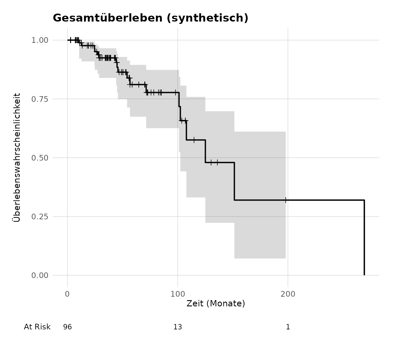

Stratified by entity, with the log-rank p-value and the median-survival reference lines:

zhn_plot_km(cohort, time_col = "os", event_col = "death_event",
            group_col = "geschlecht", show_pvalue = TRUE, show_median = TRUE,
            title = "Gesamtüberleben nach Geschlecht")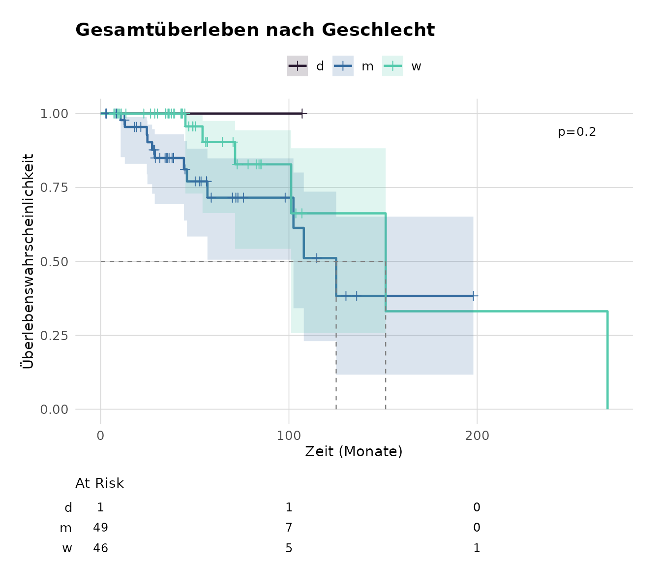

For a two-group comparison, show_hr = TRUE adds the Cox hazard ratio with its 95% CI. The hazard ratio always ships with a survival::cox.zph() proportional-hazards check: when the assumption looks violated, a caution note is added to the caption rather than reporting the HR silently.

Oncoprint table

onco <- zhn_parse_oncoprint(cohort)
onco |>
  dplyr::select(patient_label, diagnose_label, alteration, alteration_class) |>
  dplyr::slice_head(n = 6)
#> # A tibble: 6 × 4
#>   patient_label    diagnose_label        alteration alteration_class            
#>   <chr>            <chr>                 <chr>      <chr>                       
#> 1 Muster, Fall 001 Marginalzonen-Lymphom FLT3-ITD   Strukturell/Zytogenetik: De…
#> 2 Muster, Fall 001 Marginalzonen-Lymphom NRAS       Mutation/Variante           
#> 3 Muster, Fall 002 DLBCL                 KRAS       Mutation/Variante           
#> 4 Muster, Fall 002 DLBCL                 FLT3-ITD   Strukturell/Zytogenetik: De…
#> 5 Muster, Fall 002 DLBCL                 TET2       Mutation/Variante           
#> 6 Muster, Fall 003 Multiples Myelom      FLT3-ITD   Strukturell/Zytogenetik: De…

Launching the dashboard

zhn_run_app()

Use of LLM tools

Large language model tooling assisted with narrowly defined, non-authorial tasks only: copyediting, prose smoothing, Markdown/LaTeX formatting, scaffolding of boilerplate files (CI configs, build scripts), and code refactoring. The tools were Chat AI (the LLM service of KISSKI, GWDG) and a self-hosted Mistral Small (24B, Apache-2.0) run locally via Ollama and the ollamar R package — local inference only, with no data sent to third parties for the self-hosted model.

All scientific claims, methodological choices, analyses, interpretations, and conclusions are the author’s own. No LLM-generated text was incorporated without review and revision, and every reference was verified against its DOI, arXiv ID, or ISBN.